Editor’s Note: This post highlights data from Webb science in progress, which has not yet been through the peer-review process. These results were reported as part of NASA’s role in the International Asteroid Warning Network.
NASA’s James Webb Space Telescope recently turned its watchful eye toward asteroid 2024 YR4, which we now know poses no significant threat to Earth in 2032 and beyond.
We spoke with Andy Rivkin of the Johns Hopkins University Applied Physics Laboratory, the principal investigator of the Webb Director’s Discretionary Time program used to study the asteroid’s characteristics from the observations.
What is important for people to know about these Webb observations?
While earlier in the year asteroid 2024 YR4 posed a potential future impact threat to Earth in 2032, by the end of February, NASA announced the risk of Earth impact had been significantly lowered to near-zero. Nevertheless, we are interested in using the observatory to measure its properties to understand what asteroids of this size are like to help inform the hazard they could pose to Earth. This is the smallest object targeted by the mission to date, and one of the smallest objects to have its size directly measured.
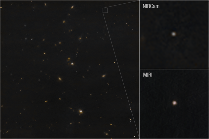
Why did you request to use both NIRCam (Near-Infrared Camera) and MIRI (Mid-Infrared Instrument) in this investigation? What did each tell you?
Most telescopes observe asteroids by measuring sunlight reflected from their surfaces, and it’s hard to precisely determine their sizes from this information. At mid-infrared wavelengths like those used by MIRI, however, the heat given off by asteroids themselves can be measured and used to directly give the asteroid’s size. The NIRCam data covers the reflected light, and using it along with the MIRI data gives us not only the size but also a measure of how reflective its surface is, which is related to the asteroid’s composition.
The chance of Asteroid 2024 YR hitting Earth in 2032 has greatly decreased, according to NASA’s Planetary Defense Coordination Office. Why are these observations still important?
While we are confident that 2024 YR4 will not hit Earth in 2032, there is still great value in making these observations and analyzing the results. We expect more possible impactors to be found in coming years as more sensitive asteroid search programs begin operation. Observations using the most powerful telescope we have right now are invaluable. Understanding the best ways to use it and how to get the most out of its data is something we can do now with 2024 YR4. This will help us determine the best approach to use during a more urgent observing program should another asteroid pose a potential impact threat in the future.
What have you learned? Was there anything surprising about the data?
We found that the thermal properties of 2024 YR4, in other words how quickly it heats up and cools down, and how hot it is at its current distance from the Sun, are not like what we see in larger asteroids. We think this is likely a combination of its very fast spin and a lack of fine-grained sand on its surface. We’ll need more data to say for sure, but it seems consistent with a surface dominated by rocks that are maybe fist-sized or larger. And of course, our main goal was measuring the size of 2024 YR4, which we estimate at about 60 meters (200 feet). That’s just about the height of a 15-story building.
How do the Webb observations fit within the larger picture of the study of this asteroid (and other near-Earth asteroids)?
2024 YR4 and other near-Earth asteroids are studied by NASA’s planetary defense program and the international community of astronomers, orbit calculators, and impact physicists, among other scientists involved in the International Asteroid Warning Network. The new observations from this observatory not only provide unique information about 2024 YR4’s size. They also added to ground-based observations of 2024 YR4’s position to help improve our knowledge of its orbit and future trajectory. Some colleagues were also able to use other telescopes to make measurements of 2024 YR4’s spin rate and spectral properties shortly after it was discovered. All together, we have a better sense of what this building-sized asteroid is like. This in turn gives us a window to understand what other objects the size of 2024 YR4 are like, including the next one that might be heading our way!
About the Author
Andy Rivkin, a planetary astronomer at the Johns Hopkins University Applied Physics Laboratory, is the principal investigator of the Webb Director’s Discretionary Time program used to study asteroid 2024 YR4.
Related Links
![Images of the trans-Neptunian objects (TNOs) Pluto [left] and Arrokoth [right], the primary flyby targets of NASA’s New Horizons spacecraft in 2015 and 2019.](https://blogs.nasa.gov/webb/wp-content/uploads/sites/326/2025/02/sidebyside.png?w=840)