sreiny – Page 4 – NASA Earth Expeditions

Five Ways Hurricanes Have Affected Puerto Rico’s Forests

A stream cuts through El Yunque National Forest in northeastern Puerto Rico. The image, captured in May 2018 by Goddard’s Lidar, Hyperspectral, and Thermal Imager (G-LIHT), reveals an open canopy. The forest floor, once cloaked in heavy shade before Hurricane Maria, now receives direct sunlight. Credit: NASA

by Samson Reiny / PUERTO RICO /

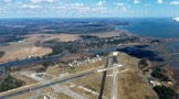
Last September 2017, Hurricanes Irma and Maria hit Puerto Rico, knocking out critical infrastructure and ransacking the island’s forests. This April and May, a team of our scientists took to the air to take three-dimensional images of Puerto Rico’s forests using Goddard’s Lidar, Hyperspectral, and Thermal Imager (G-LIHT), which uses light in the form of a pulsed laser. By comparing images of the same forests taken by the team before and after the storm, scientists will be able to use those data to study how hurricanes change these forest ecosystems.

Here are five ways scientists say the hurricanes have changed Puerto Rico’s forests since making landfall eight months ago:

1. The Canopy Is Bare

The now open canopy in Puerto Rico’s El Yunque National Forest. Credit: NASA/Samson Reiny

One word defines the post-hurricane forest canopy in El Yunque National Forest: Open.

“The trees have been stripped clean,” said NASA Goddard Earth scientist and G-LiHT co-investigator Doug Morton, who returned to the forest in April to gather measurements of trees on the ground to complement the airborne campaign’s lidar work. He was there a year ago, months before the hurricanes would ravage the area. He pointed out that from the mountainside he could see downtown San Juan, which is 45-minutes away by car.

And no canopy means no shade. “Where once maybe a few flecks of sunlight reached the forest floor, now the ground is saturated in light,” Morton said, adding that such a change could have profound consequences for the overall forest ecosystem. For example, some tree seedlings that thrive on a cool forest floor may whither now that daytime temperatures are as much as 4 degrees Celsius (7 degrees Fahrenheit) hotter than they were before the hurricane. Meanwhile, as we shall see, other plants and animals stand to benefit from such changes.

“Who are the winners and losers in this post-hurricane forest ecosystem, and how will that play out in the long run? Those are two of the key questions,” said Morton.

2. Palms Are on the Rise

Sierra Palms withstood the powerful hurricane winds better relative to hardwood tree species. Credit: NASA/Samson Reiny

One species that’s basking in all that sunlight is the sierra palm, said Maria Uriarte, a professor of ecology at Columbia University who has researched El Yunque National Forest for 15 years. “Before, the palms were squeezed in with the other trees in the canopy and fighting for sunlight, and now they’re up there mostly by themselves,” she said. “They’re fruiting like crazy right now.”

The secret to their survival: Biomechanics.

“The palm generally doesn’t break because it’s got a flexible stem—it’s got so much play,” Uriarte said. “For the most part, during a storm it sways back and forth and loses its fronds and has a bad hair day and then it’s back to normal.” By contrast, even neighboring trees with very dense, strong wood, like the Tabonuco, were snapped in half or completely uprooted by the force of the hurricane winds.

“Palm trees are going to be a major component of the canopy of this forest for the next decade or so,” added Doug Morton. “They’ll help to facilitate recovery by providing some shade and protection as well as structure for both flora and fauna.”

3. Vines Are Creeping Opportunists

Lianas are woody vines that climb trees and compete with them for sunlight at the canopy level. Credit: NASA/Samson Reiny

Rising noticeably from the post-hurricane forest floor of El Yunque National Forest are woody vines called lianas. Rooted in the ground, their goal, Morton says, is to climb onto host trees and compete for sunlight at the top. That, combined with the fact that their weight tends to slow tree productivity potential, means they are literally a drag on the forest canopy. As lianas can wind their way around several trees, regions with more of these vines tend to have larger groupings of trees that get pulled down together.

“There’s some indication that vines may be more competitive in a warmer, drier, and more carbon dioxide-rich world,” Morton said. “That’s a hypothesis we’re interested in exploring.”

4. Endangered Parrot Populations Took a Hit

The Iguaca parrot is the only native parrot left in Puerto Rico and is an endangered species. Credit: U.S. Fish and Wildlife Service/Danna Liurova

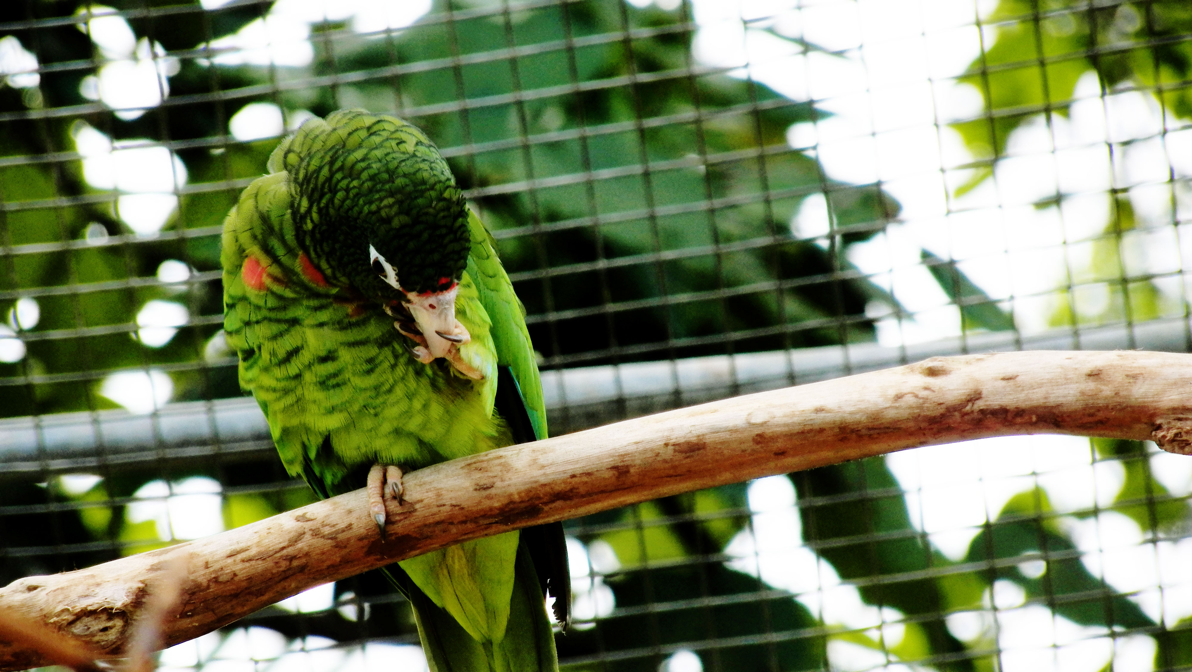
The Iguaca is the last living native parrot species of Puerto Rico. Deforestation from agriculture brought the population to its knees, but as forests have reclaimed much of the land over the past 50 years, the U.S. Fish and Wildlife Service’s Iguaca Aviaries have been working to restore their numbers by breeding and releasing the parrots into the wild.

The island’s two Iguaca aviaries have reported a substantial number of deaths in the wild due to the hurricanes. In the forests of Río Abajo, in western central Puerto Rico, about 100 of the roughly 140 wild parrots survived; in El Yunque National Forest in the eastern part of the island, only three of the 53 to 56 wild parrots are known to have pulled through.

“It was a huge blow,” said the U.S. Fish and Wildlife Service’s Tom White, a parrot biologist stationed at the aviary in El Yunque, which took the brunt of Hurricane Maria’s Category 5 winds. Some of the parrots died during the storm—from being thrashed around or being hit by falling tree limbs, for example, while others likely died from increased predation from hawks because there were no longer canopies for them to hide in. The rest succumbed to starvation. The Iguaca subsists on flowers, fruits, seeds, and leaves derived from more than 60 species—but for several months following the storm, the forest was completely defoliated.

Despite the setback, White said he’s optimistic that the Iguaca will rebound. In Río Abajo, the number of wild Iguaca are enough that they should rebound on their own. In El Yunque there are about 227 birds at the aviary—a strong number for continued breeding and eventual release into the forest once conditions improve enough. “One of their main fruit comes from the sierra palm, and they’re now flowering and starting to produce again,” White noted. “It’s probably going to take about another year for things to level out, but the forest is gritty.”

5. Lizards and Frogs: A Mixed Response

When Hurricane Maria stripped the leaves off of trees, changes in the forest microclimate instantly transformed the living conditions for lizards and frogs. Species have reacted differently to the event based on the conditions they are adapted to, said herpetologist Neftali Ríos-López, an associate professor at the University of Puerto Rico-Humacao Campus.

This adult Emerald Anole lizard was found on a tree trunk close to the forest floor. The species traditionally prefers the canopy for its dryness and warmth, but defoliation from the hurricanes have extended that type of microclimate all the way to the forest floor. Credit: NASA/Samson Reiny

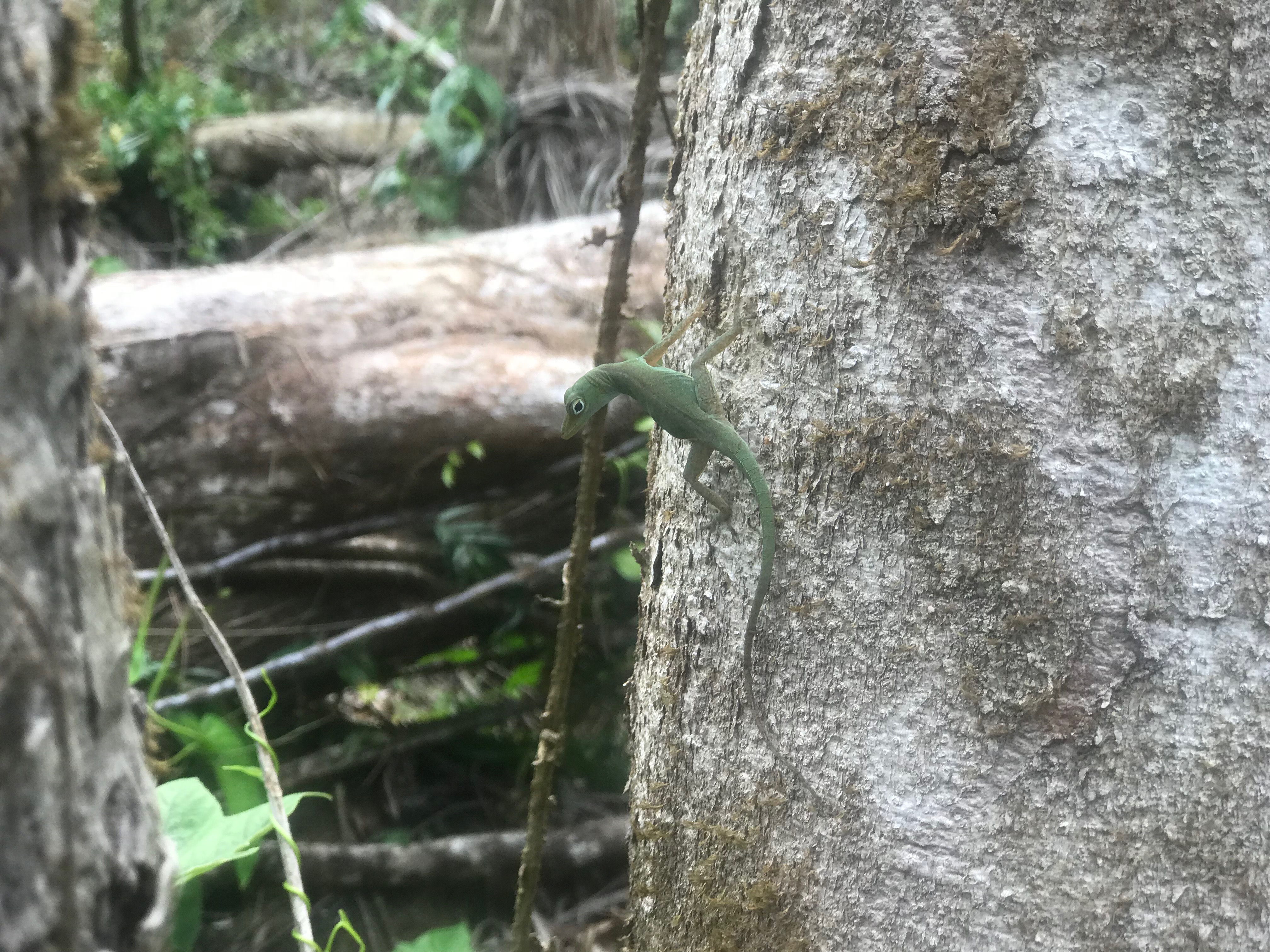
For example, some lizard species are naturally suited to the forest canopy, which is warmer and drier. “After the hurricane, those conditions, which were once exclusive to the canopy, have now been extended down to the forest floor,” Ríos-Lopez said. “As a result, these lizards start displacing and substituting animals that were adapted to the once cooler conditions on the forest floor.”

The Red-eyed cocqui’s ability to live in dry, warm areas has allowed the species to expand their range to higher elevation forests. Credit: U.S. Geological Survey

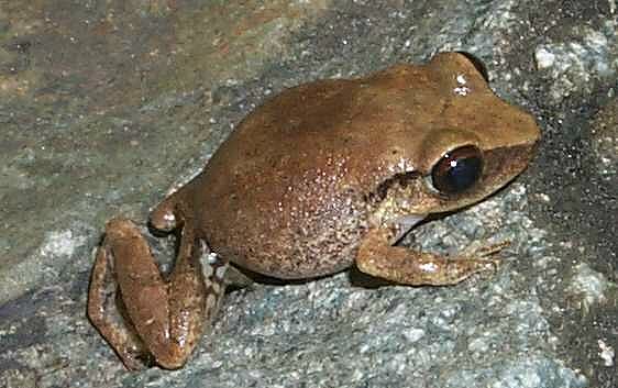
Coqui frogs, notable for their bisyllabic chirps, are the dominant frogs in Puerto Rico, which is home to 17 coqui species. Among them, the red-eyed coqui, with its resistance to temperature and humidity fluctuations and its ability to handle dehydration better than other species, has benefited from the warmer, drier conditions in the forests after the storm. Traditionally a grassland species, they are expanding from the lowlands to the middle and higher parts of the mountains, Ríos-Lopez said. “Physiologically, what was a disadvantage for that species when the whole island was forested now finds itself in a positive position.” Conversely, forest-acclimated coqui frog species have declined.

All that being said, complexities abound, cautioned Ríos-Lopez. Hurricane Maria seems to have had little impact on some coqui species that live on the forest floor despite the increases in temperature and the drier air, for instance. And before Maria, another major event occurred that will have to be counted as a factor in the current landscape: a drought that lasted from 2015 to 2017. “Many of these animals were also suffering from the drought, particularly the upland forest frogs,” he said. “That event is working in synergy with the impacts from Hurricane Maria.”

That said, as the forests recover, so will many of the species whose numbers have dwindled following the storms. “It will take many years, decades, I would guess,” Ríos-Lopez said.

Our scientists are working with partners from universities and government to use G-LiHT data to inform ground research on forest and other ecosystems not only in Puerto Rico but also throughout the world. To follow their campaigns and keep up with the latest news, find them here: https://gliht.gsfc.nasa.gov.

Cloudy with a Chance of Chemistry

The Atmospheric Tomography, or ATom, mission is investigating the atmosphere above the remote oceans. Above the Atlantic ocean near Ascension Island, the research team saw haze from African fires during ATom’s February, 2017, flight. Credit: NASA

by Ellen Gray

The most important question at the daily briefing for NASA’s Atmospheric Tomography, or ATom, mission is: What are we flying through next?

For the 30 scientists plus aircraft crew loaded up on NASA’s DC-8 flying research laboratory on a 10-flight journey around the world to survey the gases and particles in the atmosphere, knowing what’s ahead isn’t just about avoiding turbulence. It’s also about collecting the best data they can as they travel from the Arctic to the tropics then to the Antarctic and back again.

ATom’s flight path over the oceans. Credit: NASA

“ATom is all about the up and downs,” said Paul Newman, lead of the ATom science team and chief scientist for Earth Sciences at NASA’s Goddard Space Flight Center in Greenbelt, Maryland. The ups and downs he’s referring to are slow descents from 40,000 feet to 500 feet above the ocean so the researchers aboard can sample the atmosphere at all altitudes in between. That’s not a maneuver the pilots will do if they can’t see what’s below or ahead of them, but the measurements are why the team is out there.

The DC-8 makes a series of dips to the surface during each leg of the flight to sample air at all altitudes. Credit: NASA

Which is why to find out what they might encounter and safely plan their flight path, it takes a team back home in their offices supporting them with freshly downloaded satellite data, updating forecasting models, an internet connection and phone. The pre-flight briefing takes place at 9 a.m. where the plane is, so for the forecasters calling in from Colorado, Virginia, and Maryland, it often means working late or early to brief the mission scientists and pilots at their hotel. And then when the flight takes off, one of them is in the plane’s private satellite chat room giving them live updates while the plane is in the air.

Weather is of course the big concern. The pilots of the DC-8, which in another life was a mid-sized passenger plane, need to know where the fair and foul weather is.

“Just cutting across the equator, what do you do?” Newman said. “You just fly through those thunderstorms? Or is it better to go west or east around a particular convective cell? You don’t want to get trapped. We don’t want to spend a lot of time flying through a thick cloud. It screws up your measurements, clogs up your air intakes. So with real-time meteorological support, it creates a level of comfort for the team and pilots to know that there won’t be any surprises.”

View from the DC-8 above the Pacific Ocean, Feb. 2017. Credit: NASA/Róisín Commane

Weather isn’t the only forecast the team gets before and during the flight. They also get a forecast of the atmospheric chemistry. From supercomputers at Goddard, a computer simulation of Earth projects the paths of carbon monoxide plumes. Carbon monoxide is one of over 400 gases being measured aboard the DC-8, but since it’s the result of incomplete combustion, whether from cars, power plants, wild fires or agricultural fires, it’s one of the simplest for the computer to track. Like a weather forecast, the chemical forecast takes current satellite data of carbon monoxide and then uses winds and temperature to project where it will go into the future – and where the DC-8 aircraft might encounter it on flight day.

“It’s fun to see during the flight whether or not some of these forecasts are realized,” said Julie Nicely of the chemical forecast team. “The person who measures carbon monoxide, for instance, might get on the chat and say, ‘Oh, we just saw CO [carbon monoxide] rise right where you said it would!'” Where turns out to be the easier question to answer. How much of it there is and what other gases occur with and react with it to turn into other gases are much more difficult questions and are among the reasons ATom’s science team is flying through these plumes of pollution.

Carbon monoxide isn’t the only gas whose intermingling with other atmospheric chemistry is being studied. When Nicely’s not supporting ATom she’s researching the hydroxyl radical, a chemical that lasts for a fraction of a second before reacting with other gases in the constantly churning chemistry of the atmosphere. It’s impossible to simulate in the model at the moment, and ATom’s flights are the first time its concentration, along with hundreds of other gases, is being measured on a global scale.

What the science team learns from these flights will go toward not only understanding the chemistry along the strip of the ocean their plane flew over but also improving the atmospheric chemistry models that are a tool for looking at what’s happening across the entire globe.

Team Sea Ice or Team Land Ice?

Above Greenland, where land ice meets sea ice and some open water. Credit: NASA/Linette Boisvert

by Linette Boisvert / Kangerlussuaq, Greenland /

For more about Operation IceBridge and to follow future campaigns, visit: http://www.nasa.gov/icebridge

I am lucky enough to get to travel to Kangerlussuaq—a small town on the southwestern coast of Greenland that means “big fjord” in the Kalaallisut language—to join NASA’s Operation IceBridge for the remainder of their Arctic spring campaign.

Map of Greenland showing the location of Kangerlussuaq. Credit: Google Maps

I landed in Kanger on the morning of Friday, April 20, after leaving Washington, D.C., Wednesday evening, flying and overnighting in Copenhagen, Denmark, and then taking an Air Greenland flight, crossing the Atlantic Ocean twice in less than 36 hours. (Fun Fact: Greenland is owned by Denmark, so flying through Copenhagen is the only way to get to Greenland commercially.) The flight was on an Airbus, which had a surprisingly large number of passengers aboard.

After landing I thought, hmm, why do all of these people want to go to Kanger? Kanger is a small, roughly 500-person town comprising buildings surrounding the airport. There is a grocery store, a coffee/ice cream shop that never appears to be open, a youth “jail” for all of Greenland, and a Thai restaurant that is known for its pizza. Odd.

View of the town of Kanger from across the river. Credit: NASA/Linette Boisvert

Regardless, Kanger is pretty, being situated in the fjord valley with a river running through it, although currently it is frozen solid. It is also warmer here than I would have expected for Greenland, with highs in the upper 20’s to low 30’s. For the rest of the campaign, until May 4, I will be in Kanger, with the rest of my “OIB family,” as I call them, living in dorm-style housing and cooking family-style dinners together just about each night.

Build your own pizza for dinner in our dorm-style housing in Kanger. Credit: NASA/Linette Boisvert

April 21 was our first science flight out of Kanger, and as with the rest of the flights from here, it was a land ice flight. Sidebar: I am a sea ice scientist and have never been on a land ice flight before. There is a friendly rivalry between the land ice and sea ice scientist community (go Team Sea Ice!), and it is clear here that I am the only sea ice fanatic aboard, so I get picked on a bit. For those of you who don’t know, sea ice is frozen seawater that floats around on the ocean, and land ice is snow that is compacted over many, many years and turns into ice and is located on the bedrock of Greenland. Sea ice = salty (good in a margarita), while land ice = fresh (good in a smoothie).

NASA P-3 aircraft propellers outside the hangar in Kangerlussuaq, Greenland. Credit: NASA/Linette Boisvert

Photo showing land ice (bottom left corner) flowing down through the channel in the (center), and sea ice (bottom right corner). Credit: NASA/Linette Boisvert

It is not surprising to say that they really wanted to convert me to Team Land Ice, and they couldn’t have chosen a more scenic flight for this attempt. The flight is named Geikie 02 and highlights eight glaciers on the Geikie Peninsula on the eastern coast of Greenland.

Screen shot of the “Geikie 02” flight line mid-flight. Credit: NASA/Linette Boisvert

Glaciers are slow-moving rivers of ice, where land ice from the Greenland Ice Sheet is transported into the oceans or sea ice pack depending on location and time of year. As the ice gets forced into these channels and around bends, it cracks, making crevasses, similar looking to crocodile skin (or the skin on your elbow) at times.

Crevassed land ice in the foreground and Greenland mountains behind. Photo credit: NASA/Linette Boisvert

These glaciers have carved out deep channels and fjords in the bedrock over time, making for awe-inspiring views and terrain, especially when you are flying in the P-3 plane at just 1500 feet. There were many times where I would look out the window and see mountains reaching high above us as we flew over the glaciers deep in the fjord valleys and other times where it felt as it we were just skimming the tops of the mountains. This is not something that normally happens on commercial airline flights and is not for the faint of heart, but it is spectacular to behold, and I felt truly lucky to be able to witness this magnificent place.

As we flew out of the fjord to where both land ice and land meets sea, I instantly became overjoyed to view the sea ice (go Team Sea Ice!): all thicknesses, broken up, ridged, consolidated and flooded along with numerous leads and icebergs, which are land ice deposited into the ocean from the glaciers. Sea ice on a land ice flight? I think I could get used to this.

An iceberg surrounded by sea ice. Credit: NASA/Linette Boisvert

Sea ice floes, openings, and leads. Photo credit: NASA/Linette Boisvert

Where sea ice meets Greenland’s cliffs and mountains. Credit: NASA/Linette Boisvert

As we crossed the fjords and the sea ice, we noticed multiple polar bear tracks in the snow (likened to a “polar bear highway”), and multiple holes in the sea ice where seals will come out for air and rest. A few people even claimed they saw a polar bear running on the sea ice after being startled by our plane flying over, but I didn’t see it and I am skeptical. Another highlight of this flight was flying past Greenland’s tallest mountain, Gunnbjorn, which rises 12,000 feet, and the “Grand Canyon of Greenland” – the one not covered by kilometers of ice in the center of the ice sheet that data from a previous IceBridge campaign had recently discovered. Needless to say, I was glued to my window for the majority of this flight. These pictures just don’t do them justice.

Flying in a fjord valley with the mountains above us. Credit: NASA/Linette Boisvert

Although this flight did not convert me to Team Land Ice, it did reiterate to me that all ice types matter, especially in the broader context of climate change, and it is the main reason for the IceBridge field campaign: to repeatedly gather data of both land and sea ice to determine where, how, and why both ice types are changing. Specifically, melting land ice flows into the ocean and contributes to global sea level rise, whereas the loss of sea ice affects ocean and atmospheric circulation patterns both locally and globally, reminding us that what happens in the Arctic doesn’t stay in the Arctic.

Operation IceBridge Test Flights Part 2: From ‘Sick Sacks’ to Cloud Nine

NASA’s P-3 Orion research aircraft landing back at NASA Wallops Flight Facility. Credit: NASA/Aaron Wells

by Linette Boisvert / NASA WALLOPS FLIGHT FACILITY, VIRGINIA /

Linette Boisvert is a sea ice scientist at NASA’s Goddard Space Flight Center in Greenbelt, Maryland, and researcher with Operation IceBridge. The mission of Operation IceBridge, NASA’s longest-running airborne mission to monitor polar ice, is to collect data on changing polar land and sea ice and maintain continuity of measurements between ICESat missions. This blog describes test flight activities before the mission’s spring Arctic ice survey, which began on March 22 and will be ongoing through most of April.

For more about Operation IceBridge and to follow future campaigns, visit: http://www.nasa.gov/icebridge

Thursday, March 15, 2018

I woke up not as optimistic as the morning before. With the previous flight’s turbulence and motion sickness, I was not looking forward to some of the maneuvers that we were going to do. But I reluctantly went back to Wallops and got back on NASA’s P-3 Orion research aircraft. The plane was a lot less crowded for the radar test flights. A few of my friends poked fun at my vomiting on the previous flight, and I jabbed back, saying, “Take a cookie, they taste just as good going down as they do coming back up.” Yes, I still had cookies to dole out. After this, I immediately went to the cockpit to apologize to the pilots and flight engineer for puking where they work.

The P-3 Orion hanger at NASA Wallops Flight Facility. Credit: NASA/Linette Boisvert

This flight was to test the Center for Remote Sensing of Ice Sheets (CReSIS) radar. The CReSIS radar on OIB is used to determine the thickness of the snow pack on top of the sea ice and the different accumulated layers of snow on the Greenland Ice Sheet. The flight would be six hours in duration and would fly south to Norfolk, Virginia, then turn due east and head 200 miles out to sea to do the maneuvers that were required by the radar teams. These maneuvers consisted of slow rolls, quick, 60-degree rolls at 1 degree per second, and elevation-change maneuvers (ups and downs). Those aboard assured me that this flight would be much smoother due to the higher altitude (~20,000 feet) and the fact that we would be flying over the ocean.

They did not disappoint! This flight was smooth and unlike any flight I have ever experienced. I spent a lot of time in the cockpit for the best views and also because it was much warmer there than the rest of the plane. I must admit, I was a little nervous that I might have motion sickness again, but thankfully I did not. I began talking with the P-3 flight engineer Brian Yates and he let me sit in his seat for about 30 minutes. This is the best seat in the house—in the middle of the cockpit—and might I add that it reclines! This is a luxury not afforded to ANY of the other seats on the P-3.

Lynette Boisvert smiles for the camera while in the flight engineer’s seat in the cockpit of the P-3.
Credit: NASA/Jeremy Harbeck

The first time they did a rolling maneuver you could feel the g-force on you, and as the blood was being pushed from your head, it felt as if you could not move your feet from the ground. It was a very interesting feeling and I felt a little like an astronaut. For the faster, 60-degree rolls, they had me stay in the cockpit. I was a little nervous for what I was in for.

Pilot Mike Singer executing a 60-degree roll maneuver. Credit: NASA/Jeremy Harbeck

These rolling maneuvers were kind of like being on a carnival ride, and the back-and-forth lulling motions kind of made me feel like I was being rocked to sleep. During this time, I looked back from the cockpit into the rest of the plane and noticed on John Sonntag’s computer our flight line, or as John puts it, “the pilots are drunk” type of flight path, and laughed.

The P-3’s propellers during a rolling maneuver. Credit: NASA/Jeremy Harbeck

The flight path during the roll maneuvers.
Credit: NASA/John Sonntag

Afterward were the up and down maneuvers at different elevations. Again, I was seated in the cockpit, and this felt more like being on a rollercoaster. What I thought was the most interesting aspect of this maneuvering was flying into the cumulus—puffy, cotton candy clouds—and getting to experience it head-on from the cockpit. The updrafts and downdrafts present in the clouds, produced by the mixing of air causing condensation and creation of water droplets to sustain themselves, made for a little turbulence, although nothing like what was witnessed on the prior flight. During landing I was able to sit on my ledge in the cockpit, which is always a thrill. Luckily, the landing was smooth and we were back at Wallops Flight Facility.

Throughout all of this the CReSiS radar teams were working frantically, all huddled around the workstation of remote sensing expert John Paden from the University of Kansas. It appeared as if they were having problems, but if they were, they must have resolved any issues because radar data were successfully collected and calibrated during the flight.

As Melinda and I drove back to NASA Goddard Space Flight Center, located in the concrete jungle of the D.C.-Maryland suburbs, much different from the coastal, rural area surrounding Wallops, we reminisced how much fun the test flights were and how it is always so fascinating to see exactly how the instrument teams work and how the data are collected—data that we use to study the rapidly changing conditions of the Arctic sea ice.

It is also so inspiring to see how dedicated these people are to their jobs and to the OIB mission itself. They spend multiple months away from home in the Arctic and Antarctic, collecting data for scientists and the public to use. During this time they become a family, a cohesive unit, working together to complete successful flights. In some ways, they are like P-3 cowboys riding into the great unknown, wrangling this vastly important data for those of us sitting behind a desk on the ground to use and study. They are the true heroes, and for this we are truly grateful.

Operation IceBridge Test Flights Part 1: ‘Sick Sacks’ for Science

Sunrise from over Wallops Island. Photo credit: NASA/Linette Boisver

by Linette Boisvert / NASA WALLOPS FLIGHT FACILITY, VIRGINIA /

For more about Operation IceBridge and to follow future campaigns, visit: http://www.nasa.gov/icebridge

And click here for part 2 of Linette’s blog.

Wednesday, March 14 2018

Kyle Krabill calibrating GPS on the P-3. Photo credit: NASA/Jeremy Harbeck

I woke up early Wednesday morning at our shared “beach house” to make coffee and was greeted with a beautiful sunrise from the front porch over Wallops Island and the NASA water tower in the distance. Sipping on my coffee, I had high hopes that this was going to be a great day. Coincidentally, Kyle Krabill, Airborne Topographic Mapper (ATM) ground GPS guru, and John Sonntag, the legend and the man behind why the Operation IceBridge (OIB) missions run so smoothly, were at the Wallops Flight Facility doing a calibration of the NASA P-3 Orion research aircraft’s GPS antenna.

My colleague and friend Melinda Webster and I arrived at Wallops at 8 a.m. on this clear, brisk and windy morning, driving around the grounds trying to find the D-1 hangar. However, it didn’t take us long to find it, as we saw the tail of the P-3 sticking above a few buildings. We headed over and immediately saw Jeremy Harbeck, OIB’s resident photographer, data analyzer and pun-master coming out of the hanger door with a big smile on his face to greet us. Inside, we watched an informative, somewhat corny pre-flight safety video (don’t wear open-toed shoes or heels on the plane) before the flight.

NASA’s P-3 Orion research aircraft on the tarmac at WFF. Credit: NASA/Jeremy Harbeck

After the video, we were free to board the plane, and as we walked on the tarmac, careful to mind the P-3’s propellers, we noticed the wind had picked up significantly. In hand, I carried homemade sugar cookies shaped like airplanes, decorated in red and green icing with words like “ATM” and “OIB”; red and green to signify the red and green lasers on the ATM. With these cookies, I was determined to win over the instrument team members, pilots and flight crew who I did not know well and to put smiles on everyone’s faces. I wanted to come out of my shell and get to know everyone and learn how the teams worked. As I was handing out cookies, each engineer and flight crew stopped what they were busily working on to chat and munch on the cookies before getting back to it. Everyone on the plane was frantically working and knew what they had to accomplish before the flight. As we were hanging out in the plane we noticed that the strong winds that had picked up since the early morning were causing the plane to shake. No big deal, we thought.

Homemade airplane cookies. Credit: NASA/Linette Boisvert

Pre-flight activities aboard the P-3. Credit: NASA/Linette Boisvert

The day’s two-hour flight would be to test the ATM lasers and the Digital Mapping System (DMS) camera in order to make sure that they were calibrated in the air on the plane for the science flights over Arctic sea ice and the Greenland Ice Sheet. We would fly 1,500 feet above the surface along the coast to Bethany Beach, Delaware, back south over the ocean to a buoy measuring wave height (for scientists at the University of Washington’s Polar Science Center, because science never stops, after all), and then a series of six “ramp passes” at different altitudes over the Wallops Flight Facility runway, where highly accurate ground GPS surveys have been taken for calibration. ATM surface elevation data are used to infer the thickness of the sea ice pack from the “freeboard”—how high the Arctic sea ice extends above the ocean surface—and for surface elevation changes and mass loss from the Greenland and Antarctic Ice Sheets.

View of the Atlantic Ocean and eastern Shore of Maryland.
Photo credit: NASA/Linette Boisvert

The P-3 took off as it normally would, as I’ve been on it a few times before with OIB, with a little bumpiness; however, once we were up at 1,500 feet the turbulence did not go away. Not thinking much of it, Melinda and I had moved to a window to watch the coastline below (it was very odd to NOT view sea ice out of the P-3 window) when I began to feel a little bit funny, despite everyone around me looking fine and happy.

NASA Wallops Flight Facility during a ramp pass. Credit: NASA/Alexey Chibisov

Now, flights over sea ice are not very turbulent because the boundary layer over the ice is often very stable due to the small contrast in temperatures between the cold ice surface and cold air above. However, 1,500 feet above the land and so near the Atlantic Ocean, there are drastic temperature differences between these surfaces, both ocean and land and also the air above. Mix that with strong winds and sunny conditions warming the surface, and you get thermals and instability with the air in the boundary layer. In simple terms, this means lots of turbulence, and lets just say I was not used to it.

So I was beginning to feel pretty queasy, and I was wondering what this feeling was since I have never experienced motion sickness before. I tried not to think about it and snapped a few photos of the coastline and of some ATM instrument team members lying on the floor of the P-3 reaching underneath the floor to performing an optical alignment of the T7 ATM laser. (This photo would be likened to a crime scene photo. What do you think?)

‘Crime Scene’ ATM team members hard at work in flight. Credit: NASA/Linette Boisvert

Taking pictures was not making the feeling in my stomach go away. With this feeling growing worse, I asked Melinda, still smiling and happy, if she could find me a container to “lose my breakfast” in. She came back quickly with “sick sacks,” as they are called, thanks to the quick reaction time of Michael Studinger, a seasoned ATM and airborne veteran, and I was told to go in the cockpit and look at the horizon. It supposedly helps.

So I went and sat on my ledge in the cockpit, my usual spot during normal sea ice flights, but the motion sickness feeling was not letting up. Finally, I “let it go,” as a Frozen Disney princess once said. Up came my airplane cookie, which made its way into my sick sack right there in the cockpit. How embarrassing. On top of that, I was too afraid to move. After six torturous ramp passes and unending turbulence, we finally landed back at Wallops. The turbulence was no big deal to the pilots, underscoring, again, the seasoned veterans’ expertise.

Linette Boisvert with her ‘sick sack’. Credit: NASA/Melinda Webster

Needless to say, I was not sad that this flight was over, but I was pleased to hear that all of the instruments had no problem collecting data on the flight, which in large part was due to the instrument teams’ efforts. It is also clear to see that these people love their jobs and what they do so much that they are willing to—and even often do get—motion sickness on the plane and keep on chugging along.

Observing Biodiversity: One Cell at a Time

A sample mosaic image from the Imaging FlowCytobot, representing material sampled from one bottle of seawater collected by during a CTD cast. Credit: NASA

by Eric Lindstrom / Eastern Tropical Pacific Ocean /

Eric Lindstrom is Physical Oceanography Program Scientist at NASA Headquarters. For the last 20 years, his primary job has been supporting NASA satellite missions related to measuring physical characteristics of the ocean (principally, temperature, salinity, sea level, and winds) and supporting the oceanographers that generate knowledge from such data. He was recently aboard the Research Vessel (R/V) Roger Revelle in the Pacific Ocean as part of the Salinity Processes in the Upper Ocean Regional Study-2 (SPURS-2) field campaign. SPURS is undertaking oceanographic field experiments to further understand the essential role of the ocean in the global water cycle using a plethora of oceanographic equipment and technology, including salinity-sensing satellites, research cruises, floats, drifters, autonomous gliders and moorings.

What lives below us? This is a question that mariners have wondered for ages. We no longer think of the darker answers to this question—the sea monsters, the Kraken, the great whales. For most aboard, the thinking is akin to a fisherman’s—tuna, mahimahi, sharks. But for SPURS-2, Sophie Clayton is answering this question in terms of microscopic life, namely diverse phytoplankton (plant life) and zooplankton (animal life).

Sophie is an oceanographer interested in understanding how ocean currents at all scales shape the distribution and biodiversity of phytoplankton. She uses a combination of numerical models, large-scale data analysis, and targeted observations made at sea. Her Ph.D. in Physical Oceanography from the Massachusetts Institute of Technology/Woods Hole Oceanographic Institution Joint Program. Now she is a postdoctoral fellow at the University of Washington, working extensively with observations of phytoplankton distributions made using an Imaging FlowCytobot (IFCB) that analyzes discrete samples with video and a hyperspectral optical sensor for recording the continuous optical properties of the water.

Sophie Clayton collects a 4-liter bottle of seawater for filtering. Credit: NASA/Eric Lindstrom

An IFCB is an instrument that is used primarily to count cells, but it also can detect and record information on different properties of the cells that it counts. A water sample is channeled into a thin stream that is passed in front of a laser, and the scatter and fluorescence from each cell that passes along the stream is detected and recorded. In the IFCB, the camera is triggered to take a picture only when fluorescence over a threshold value is detected. This means that the instrument only takes pictures of cells that contain chlorophyll. The images are then stored for analysis back on shore. In addition to the images that are collected, we use the optical properties of the cells (fluorescence and scatter) in the analysis.

Sophie’s work is enabled by surface water collected from the salinity snake while we are underway or from bottle samples taken during Conductivity- Temperature-Depth (CTD) casts. Similar mosaics are made from surface water every 20 minutes. Overall, there will be close to 2,000 mosaics of cellular life to examine. Samples are also held for later DNA analysis.

There are always meticulous notes to keep about samples. Credit: NASA/Eric Lindstrom

Out here, for the most part, the plankton are actually most abundant below the surface at 40-70 meters depth. Deeper down, below the surface layer mixed by the wind, life has better access to the chemical nutrients of the deep sea while still having enough light for photosynthesis. Plant life thrives in a layer that best balances the light and nutrient requirements. Of course, the grazing microscopic animals follow this layer closely. So Sophie is keen to collect water from this layer during our CTD casts. She can tell where to sample by optical properties also measured on CTD casts.

Understanding plankton abundance and diversity is a core requirement for ocean climate science. Phytoplankton are responsible for about half of all photosynthetic production on the planet. (Land plants are also responsible for about half.) It makes them a key part of the carbon cycle on the planet. Over long periods, phytoplankton can remove carbon from the upper ocean and return it to sediment for long-term sequestration. Over hundreds of thousands of years, phytoplankton act to reverse the greenhouse effect caused by pulses of carbon dioxide injected into the atmosphere by volcanoes or humans.

Phytoplankton are extremely diverse, varying from photosynthesizing bacteria (cyanobacteria), to plant-like diatoms, to armor-plated coccolithophores (drawings not to scale). (Collage adapted from drawings and micrographs by Sally Bensusen, NASA EOS Project Science Office.)

In a prior blog, I wondered about the fate of life in the sea. What would become of that abundant life with the continued impacts of ocean acidification, industrial fishing, and plastics pollution? Science struggles to make any predictions. Oceanographers particularly, because of our close affinity and observation of the sea, hope that the assaults of society on the sea do not damage its inherent ability to stabilize and heal the rapid changes overtaking the planet. Our baseline understanding of the complex marine ecosystem is still quite primitive. The kind of “survey” work that Sophie is undertaking is absolutely necessary to further our understanding of the biogeography of the ocean and how it is changing. Let’s hope she has a successful career!

A Career in Physical Oceanography

Eric Lindstrom is Physical Oceanography Program Scientist at NASA Headquarters. For the last 20 years, his primary job has been supporting NASA satellite missions related to measuring physical characteristics of the ocean (principally, temperature, salinity, sea level, and winds) and supporting the oceanographers that generate knowledge from such data. He is currently aboard the Research Vessel (R/V) Roger Revelle in the Pacific Ocean as part of the Salinity Processes in the Upper Ocean Regional Study-2 (SPURS-2) field campaign. SPURS is undertaking oceanographic field experiments to further understand the essential role of the ocean in the global water cycle using a plethora of oceanographic equipment and technology, including salinity-sensing satellites, research cruises, floats, drifters, autonomous gliders and moorings.

You can read more about SPURS field campaign through Eric’s Notes from the Field blogs.

The R/V Roger Revelle in San Diego just before departure. Credit: NASA/Eric Lindstrom

In July 1969 I was watching Neil Armstrong take his first step on the moon at Tranquility Base, like everyone else with a TV at the time. I was at USC Wrigley Marine Center on Catalina Island as a 13-year-old visiting my brother, who was spending the summer studying there. If you had asked me then if I would wind up working for NASA, I would have said, “No, I’d rather pursue oceanography!” Well, since 1997 I have been the Physical Oceanography Program Scientist at NASA Headquarters AND I am a dedicated sea-going oceanographer. It stills feels kind of crazy what comes around in life. I write my short career biography here for students who may consider working in oceanography or for NASA or both.

After graduating from Huntington Beach High School in California in 1973, I took the train across the country to begin my college career at the Massachusetts Institute of Technology. After only one semester of MIT physics and mathematics problem sets, this boy gravitated to the Department of Earth and Planetary Sciences and asked them how I would train to be an oceanographer. There were no undergraduate oceanography courses, so I was told to take physics and math (ouch!) and to get my degree in Earth Science I would have to take the required geology and geophysics courses, too. I did all that, but rocks were not my first love. Luckily, a Professor of Physical Oceanography at MIT, John Bennett, allowed me to work with him under MIT’s Undergraduate Research Opportunities Program (UROP) and sit in on his graduate level physical oceanography courses. We worked together on an analysis of the coastal boundary layer in Lake Ontario, and I co-authored a paper with him that appeared in the Journal of Physical Oceanography in the summer of 1977. UROP and that research paper were a big boost for my applications to graduate school. I still donate money annually to MIT’s UROP to honor its impact.

For graduate school I sought out a diverse set of schools: UCSD Scripps Institution of Oceanography, University of Washington, Princeton, and University of Miami. I was told that since I was at MIT, I should NOT apply to the MIT/Woods Hole Oceanographic Institution joint program (that was weird). In the end I did have choices and settled at University of Washington working with Professor Bruce Taft. It was the era of Apollo-Soyuz and USA-USSR cooperation in space and oceanography, so I embarked on studying eddies in the North Atlantic with a diverse set of US and USSR scientists. The project was called POLYMODE. It was a fun project with time at sea and lots of workshops and meetings, including a month in Moscow doing a data exchange. The connection to the space program was remote and programmatic and I hardly noticed it at the time. I received my PhD in September 1983, the day the Australian’s won the America’s Cup sailing race. I celebrated, since I had signed up to move to Australia to do oceanography (and get married!) the very next month.

Australia was a hoot! We moved to Hobart in Tasmania where the government was building a new marine science laboratory and eventually a new oceanographic research vessel as well. It was a growing field because 200-mile Exclusive Economic Zones had just been declared and Australia wanted to know all about the waters around the continent—good work for a newly minted oceanographer! The team in Hobart had me focus on the western tropical zone, including the Coral Sea, Solomon Sea, Bismarck Sea, and the circulation around Australia’s neighbor Papua New Guinea. Hardly anything was known so I worked with some of my buddies back in the USA on developing the Western Equatorial Pacific Ocean Circulation Study (WEPOCS). It was a great success! We named some new ocean currents and replaced some old stale ideas with some fresh perspective on the role of the western tropical Pacific in climate.

While in Australia in the 1980s I also became involved in the planning of a huge international experiment – the World Ocean Circulation Experiment (WOCE). My work on WOCE had the Australian government send me back to the USA to work at Texas A&M University, the U.S. WOCE Office. That certainly began returning my roots to US soil. After returning to Australia it was not long until headhunters from USA sought my return to work again in the USA at the project office in Boulder, Colorado, of the Coupled Ocean Atmosphere Response Experiment (COARE; an experiment just off the coast of Papua New Guinea). The family decision was to make a return to the USA permanent.

Boulder only lasted about 18 months and then I returned to WOCE work as U.S. WOCE Program Scientist in Washington, D.C., in 1992 as an employee of Texan A&M University but under the direction of five federal agencies (each providing 20 percent of my support). Gosh, the world is convoluted sometimes! That, for me, began “interagency cooperation” in oceanography for which I am still deeply involved. Broadly, the five agencies that fund global oceanography projects are the same now as they were then: NSF, NOAA, Navy, NASA, and Department of Energy.

Eventually, after five years working on WOCE and the new Global Ocean Observing System, I got a call from Bruce Douglas at NASA Headquarters. He was serving a stint as Physical Oceanography Program Scientist and asked me to interview as his replacement. NASA told me they were looking for someone who could integrate their oceanography (from space) into the federal family of oceanography agencies. Certainly, I had experience for that. However, I told them I had no particular experience with satellite oceanography. Their idea, and response at the time, was that they had plenty of satellite oceanographers at NASA but that it might be good for their leader to be someone who had “touched seawater” and was open to learning about the new tools for satellite oceanography. Wow, I said, you have found the right person!

So, here we are, after 20 years, I have learned my fair share of satellite oceanography and have thoroughly enjoyed NASA. I have molded NASA Physical Oceanography into a community that fully supports its satellite missions with appropriate science at sea. I hope I have helped to make satellites an everyday tool for oceanographers. The positive feedback from the community has been most humbling. I am very lucky indeed to have landed on my own Tranquility Base.

ACT-America: Settling into the Rhythm of the Field

C-130 pilots Jim Lawson, left, and Paul Pinaud during a flight. Credit: NASA/David C. Bowman

by Hannah Halliday / SHREVEPORT, LOUISIANA /

Fieldwork is my favorite part of my job. I have been working as a postdoc at NASA’s Langley Research Center in Hampton, Virginia, for a few days over a year, and I’m still not over the excitement of arriving somewhere new, ready to take measurements and run our instruments.

My background is in chemistry, but I slid into meteorology because I wanted to apply myself to environmental issues that had global impact. That decision put me on a path into the world of air quality research, and ultimately to NASA to work with airborne science. While I’m still new to flying for science, I love working with instruments and taking measurements. Being on an aircraft turns that feeling up to 11.

Atmospheric Carbon and Transport-America, or ACT-AMERICA, has been an especially cool project to be involved with because I earned my Ph.D. at Penn State, where principal investigator Ken Davis and other members of the ACT-AMERICA planning team are based. Working with ACT-AMERICA is part serious work and part fun reunion, working with people I know well on a totally new subject and project. I got to fly with the mission last spring, and I’ve come back to join them again for two weeks in Shreveport, Louisiana.

The C-130 doesn’t have many windows, but Halliday is lucky to have one beside her seat. Flights often have low-altitude runs, and offer views of the country from unique angles. This is a view of the Mississippi River from the Sunday, Nov. 5, flight. Credit: NASA/Hannah Halliday

On Saturday, Nov. 4, we took a break from flying to do instrument work and maintenance. For my group, which is tasked with the Atmospheric Vertical Observations of CO2 in the Earth’s Troposphere, or AVOCET, in-situ measurements, that meant calibrating our instruments. When we calibrate, we send our instruments gases that have a known concentration and record what our instruments measure. Doing this regularly allows us to keep track and correct for the instrument drifting over time, and to maintain the accuracy and precision of our measurements.

Hannah Halliday, right, monitors incoming AVOCET measurements during a Nov. 2 science flight. Next to her are Theresa Klausner and Max Eckle, Ph.D. students with the German Aerospace Center, DLR, which has joined the fall flight campaign to test an instrument that measures methane and ethane. Credit: NASA/David C. Bowman

Bianca Baier, a postdoctoral researcher with NOAA’s Earth Systems Research Lab in Boulder, Colorado, and Ken Davis, ACT-America principal investigator from Penn State, talk during a flight. Credit: NASA/David C. Bowman

Our two aircraft, a C-130 and a B-200, are stored in different locations when we’re at our ground sites. The calibration gas tanks are heavy, so for ease of use we’ve built our calibration gas cylinders their own little cart that they live on, which can be towed from one location to another. The cylinders are left on the cart, where we put a regulator on the calibration cylinder we want to use and run a tube into the airplane. It’s a simple solution that lets us easily and quickly use the same calibration gases on two different aircraft.

Calibration gas cylinders on their transportation cart. During a calibration, scientists use three gases with low, middle and high concentrations, and use this information to understand how the instrument will behave when it “sees” gases in the environment. Credit: NASA/Hannah Halliday

One of the reasons I love working in science is that our measurements and our work is built on a heap of clever solutions to small problems. While we also stand on the shoulders of scientific giants who had deep insights into the workings of the universe (for instance, Isaac Newton realizing that the gravity affecting an apple also affects the stars), in our day-to-day work we use the cleverness of the people who worked out the universal swage fittings, or the person who figured out how to set up our inlet system to bring air in from outside the plane when we’re at high altitude.

We’re not all brilliant all the time, but by looking at a problem long enough we can often find a clever solution to a small vexing problem (such as how to quickly transport our calibration cylinders), and that’s where our progress comes from.

On Sunday, Nov. 5, we flew a science mission, measuring the inflow of air from the Gulf of Mexico. It was a busy day for me, because I was both tending my group’s instruments and also taking flask samples for NOAA. NOAA uses glass-lined containers to trap air at specific locations on the flight track. They take these samples back to their lab in Boulder, Colorado, where they measure the greenhouse gases as well as other molecules that help determine whether samples were influenced by other sources, such as traffic or wildfires. My job was to follow their sampling plan, telling their mostly automated system when to collect a sample and coordinating with our in-flight calibrations.

Specialized inlets draw air into the instruments and have different designs based on the needs of the instruments. These inlets are located near the front of the aircraft so they don’t sample the exhaust from the engines. Credit: NASA/David C. Bowman

The flights can be quite busy, and it’s a full day of activity. For the four to five hours that a typical science flight will last, we have an additional three hours of flight prep before we take off, and a debriefing meeting once we land, plus data workup and archiving the preliminary data once we’re back in our hotel rooms.

The C-130 gets a checkup after the Nov. 5 flight. A dedicated flight team keeps the aircraft running and maintained. Credit: NASA/Hannah Halliday

It’s satisfying work, but it’s important that we have non-flight days like Saturday to catch up on our instrument maintenance as well as personal things—exercise, laundry, even sleep. When we’re in the field there’s no set schedule like when we’re in the office, and it’s important to grab that time when we can, because flight days depend on the weather, and a good measurement day waits for no scientist, not even when they have a plane!

ACT-America: Waiting for the Great Big Teaspoon in the Sky

The NASA Langley B200 sits in a hangar at Shreveport Regional Airport. It and the C-130 won’t fly today because the weather pattern is too similar to the one they flew through the day before. Credit: NASA/David C. Bowman

by Joe Atkinson / SHREVEPORT, LOUISIANA /

Brrrr.

I don’t know what I was expecting from Louisiana in late October, but I definitely wasn’t expecting cold and damp.

I’m here for the final leg of the fall 2017 flight campaign for Atmospheric Carbon and Transport-America, or ACT-America, a five-year NASA study looking at the transport of carbon dioxide and methane by weather systems in the eastern United States.

This is the third flight campaign of the study and the team has just arrived in Shreveport—home base for the next two weeks. Flight operations will be based out of Shreveport Regional Airport. Sleep operations are based at a hotel just a few minutes down the road in Bossier City.

ACT America group with the B200 King Air and C130 Hercules in Shreveport Louisiana. Credit: NASA/David C. Bowman

As I’ve already mentioned, the weather so far is pretty meh. There’s a slow-moving front to thank for that. But more on the creeping front later on. First, a little taste of ACT-America’s home for the next couple of weeks.

Shreveport is the largest city in Ark-La-Tex, a region that includes Northwestern Louisiana, Northeastern Texas and South Arkansas. It and Bossier City are divided by the Red River. Shreveport is on the west, Bossier City the east. Casinos dot the riverbank—the Horseshoe, Boomtown, Eldorado, Margaritaville, Diamond Jack’s.

It’s no big surprise that you can’t go far here without finding restaurants that have Cajun and Creole dishes on the menu. The first night in town, a contingent from the ACT-America team visits the Blind Tiger in downtown Shreveport. Steaming plates of crawfish etouffe come out of the kitchen accompanied by crusty homemade croutons and mounds of rice. There’s a dish called Cajun fried corn—breaded, deep-fried corn on the cob. Louisiana beers are on tap. Gumbo is spelled gumbeaux.

The State Fair of Louisiana is taking place in Shreveport. It claims to be the largest livestock show and carnival in the state. Rick Rowe, a reporter with the local ABC affiliate, does a segment on the morning news with a man who sells fried cheese at the fair. Rowe samples a cube that’s just been pulled from the bubbling hot oil and sounds positively ecstatic as he bites through the crispy breading.

The state fair isn’t the only thing going on, though. Another news segment has a meteorologist visiting a Bossier City shop that sells power equipment: lawnmowers, leaf blowers, generators, chainsaws. They have an event coming up called Sawdust Days. Folks who show up for Sawdust Days will be treated to a special demonstration by a man who does wood carvings with a chainsaw.

“He’s carved a lot of pieces right here,” the shop owner says, gesturing to a rustic-looking wooden bear that towers over him and the meteorologist, “so he’s pretty good at it.”

I turn off the TV and head to the airport to catch up with another guy who knows something about meteorology—Ken Davis, principal investigator for ACT-America and a professor of meteorology at Penn State University.

Weather is critical to ACT-America. In fact, it’s the reason that, on its first full day in Shreveport, the campaign is keeping its C-130 and B200 aircraft on the ground. Just the day before, as ACT-America moved from its previous homebase in Lincoln, Nebraska, to Shreveport, the aircraft passed through the very front that’s inching through Louisiana now, bringing the chilly air and rain along with it. Instruments on both aircraft measured carbon dioxide and methane levels during the transit.

“This weather is relatively similar to what we documented yesterday,” Davis says. “If we measured it yesterday, we don’t need to measure it today.”

Although there won’t be a flight today, there’s still work to do. Here, Yonghoon Choi, an instrument investigator from NASA Langley, and Max Eckle, a Ph.D. student with DLR, the German aerospace agency, help unload equipment and supplies that have been trucked to Shreveport from the previous ACT-America homebase in Lincoln, Nebraska. The fall flights are giving the DLR a chance to see how their methane- and ethane-detecting Quantum Cascade Laser Spectrometer operates in the field, while also allowing the ACT-America scientists to better zero in on methane sources. Credit: NASA/David C. Bowman

What the team will want to measure, though, is what happens to the greenhouse gases after the cold front stalls not too far south of Shreveport. There, it’ll get a push from warm, low-level air flowing in from the Gulf of Mexico and then move northeast as a warm front.

It’s a scenario that may take a couple of days to play out, so the next research flights may happen tomorrow, they may happen the day after tomorrow. The atmosphere will do what it wants to do, thank you. Davis likens it to a big cup of coffee.

“Over the timescale of days,” he stretches out days when he says it, “somebody’s stirring it with a great big teaspoon. And you’ve got to wait … every stir takes a couple of days. We want to measure different parts of that.”

Later on, at a planning meeting, they make the final decision—another down day tomorrow, then a flight the next day when the great big teaspoon in the sky has finally mixed things up just so. It’ll be a good day for airborne science.

The meeting breaks up. Folks head back to their hotel rooms.

With a free evening in front of me, I think about taking a chilly walk down the bank of the Red River to get a look at the Shreveport skyline at night. And for some reason, I’m craving a piping hot cup of coffee.

Hannah Halliday, left, a postdoctoral researcher at NASA Langley, and Bianca Baier, a postdoctoral researcher at the NOAA Earth System Research Laboratory in Boulder, Colorado, point out to Ken Davis a region where fires might make for interesting measurements. Credit: NASA/David C. Bowman

At a late-afternoon planning meeting at the hotel, ACT-America prinicipal investigator Ken Davis, left, listens as research scientist Sandip Pal discusses which day might be best to fly next. The weather pattern for the upcoming two days could be favorable for science flights. After much debate, they make the decision to give the pattern an extra day to set up before flying again. C-130 pilot Jim Lawson and mission manager Charles Juenger, far right, listen in. Credit: NASA/David C. Bowman

Searching for the Bluest Blue

by Joaquín E. Chaves-Cedeño / South Pacific Ocean /

It doesn’t take a lot of technology to see that the ocean is blue. And when it comes to the blueness of the ocean, it doesn’t get much more blue than where I am. My current home and office is the research vessel Nathaniel B. Palmer—the largest icebreaker that supports the United States Antarctic Program—which is on an oceanographic expedition across the South Pacific Ocean. On this voyage, however, the Palmer hasn’t broken any ice.

Our Global Ocean Ship-based Hydrographic Investigations Program (GO-SHIP) P06 campaign departed Sydney, Australia, on July 3, and successfully ended the first leg of this journey on August 16 in Papeete, French Polynesia, also known as Tahiti. This is where our team from NASA Goddard Space Flight Center (Scott Freeman, Michael Novak, and I) joined dozens of other scientists, graduate students, marine technicians, officers and crew members for the second and final leg that will end in the port of Valparaiso, Chile, on September 30.

The GO-SHIP program is part of the long history of international programs that have criss-crossed the major ocean basins, gathering fundamental hydrographic data that support our ever growing understanding of the global ocean and its role in regulating Earth’s climate, and of the physical and chemical processes that determine the distribution and abundance of marine life. This latter topic regarding the ecology of the ocean is what brings our Goddard team along for the ride.

The P06 ship track, for the most part, follows along 32.5° of latitude south. That route places our course just south of the center of the South Pacific Gyre—the largest of the five major oceanic gyres, which form part the global system of ocean circulation. The Gyre, on average, holds the clearest, bluest ocean waters of any other ocean basin. This blueness is the macroscopic expression of its dearth of ocean life. We have seen nary a fish or other ship since we departed Tahiti (as this is not a major shipping route). Oceanic gyres are often called the deserts of the sea. On land, desert landscapes are limited in their capacity to support life by the availability of water. Here, lack of water is not the issue. Water, however, is at least the co-conspirator in keeping life from flourishing. Physics, as it turns out, is what holds the key to this barren waterscape.

This map shows MODIS chlorophyll concentrations indicating phytoplankton, with the R/V Nathaniel B. Palmer’s ship track superimposed. The deeper blue the color the less chlorophyll there is. Credit: NASA

Due to the physics of fluids on a rotating sphere such as our planet, the upper ocean currents slowly rotate counterclockwise around the edges of the center of the Gyre—as a proper Southern Hemisphere gyre should—and a fraction of that flow is deflected inward, toward its center. With water flowing toward the center from all directions, literally piling up and bulging the surface of the ocean, albeit, by just a few centimeters across thousands of miles, gravity pushes down on this pile of water.

This relentless downward push puts a lock on life.

The pioneers of life in the ocean, tiny microscopic organisms known as phytoplankton, drift in the currents and grow on a steady mineral diet of carbon dioxide, nitrogen, and phosphorus, along with a dash of iron. (Meanwhile, they expel oxygen gas as a by-product, to the great benefit of life on Earth). Phytoplankton obtain most of their sustenance from the ocean below. What happens in this Southern Hemisphere gyre is that layers of denser water trap the nitrogen- and phosphorus-rich water to depths that are out of reach to most of the phytoplankton. And phytoplankton that do make it to that depth are too starved of sunlight to spark the engine of photosynthesis that allows them to grow.

Why are we here and where does NASA come into this story? Since the late 1970s, NASA has pursued, experimentally at first, and now as a sustained program, measuring the color of the oceans from Earth-orbiting satellites as a means to quantify the abundance of microscopic life. It’s microbiology from space, in a way. Formally, though, we call it “ocean color remote sensing.” Bound to polar orbits that allow them to scan the entire surface of the globe every couple of days, satellites whiz by at several hundred miles above the atmosphere carrying meticulously engineered spectra-radiometers, or cameras capable of measuring the quantity and quality, or color, of the light that reaches its sensors. This is where our work aboard the R/V Palmer comes into the story.

The crew prepares to deploy the radiometer from the stern of the R/V Nathaniel Palmer to measure the optical properties of the water from the surface down all the way down to the bottom of the photic zone. Credit: Lena Schulze/FSU

The data the satellites beam down from orbit do not directly measure how much plant life there is in the ocean. Satellite instruments give us digital signals that relate to the amount of light that reaches their sensors. It is up to us to translate, or calibrate, those signals into meaningful and accurate measurements of microscopic life, along with temperature, salinity, sediment load, sea level height, wind and sea surface roughness, or any other of the many environmental and geophysical variables satellite sensors can help us detect at the surface of the ocean. To properly calibrate a satellite sensor and validate its data products, we must obtain field measurements of the highest possible quality. That is what our team from NASA Goddard is here to do.

Scott Freeman of NASA works with an R/V Nathaniel Palmer crew member to prepare an optical instrument for deployment over the side of the ship to collect optical measurements. Credit: FSU/Lena Schulze

Around midday, typically the time an ocean color satellite is flying over our location, we perform our measurements and collect samples. We measure the optical properties of the water with our instruments to compare what we see from the R/V Palmer to what the satellites measure from their orbit. At the same time that we perform our battery of optical measurements, we also collect phytoplankton samples to estimate their abundance and species composition as well as the concentration of chlorophyll-a, the green pigment common to most photosynthesizing organisms, such as plants. By simultaneously collecting these two types of measurements—light and microscopic plant abundance—we are able to build the mathematical relationships that make the validation of satellite data products possible.

Mike Novack of NASA studies the optical and biological characteristics of sea water samples in the ship’s laboratory.
Credit: NASA/Joaquin Chavez

The waters of the South Pacific Gyre are an ideal location for gathering validation quality data, perhaps one of the most desirable, because there are few complicating factors and sources of uncertainty that blur the connection we want to establish between the color of the water and phytoplankton life abundance. Our measurements will extend NASA’s ocean chlorophyll-a dataset to some of the lowest such values on Earth. The water here is blue; in fact, it’s the bluest ocean water on Earth.