Ice Cap Recap

From: Kathryn Hansen, NASA’s Earth Science News Team / Cryosphere Outreach

May 16, 2011

Last month, IceBridge surveyed Sukkertoppen Ice Cap — a mass of ice southwest of the mission’s base in Kangerlussuaq, Greenland. I didn’t know what to expect from an ice cap. Would it resemble the vast, white expanse of the Greenland Ice Sheet next door?

At the surface, Sukkertoppen looked remarkably like an ice sheet. After all, both form from the accumulation of snow compacted over thousands of years. Before long we reached the rugged mountains and blue-green fjord that separates the cap from the main ice sheet, and we turned back for another pass.

On April 8, 2011, IceBridge flew a mission to coastal areas in southwest Greenland. Mountains and an open-water fjord surround one of the mission’s targets, a small ice cap called Sukkertoppen Isflade. Credit: NASA/Michael Studinger

Ice caps are simply small versions of ice sheets, measuring in at a maximum area of 50,000 square kilometers (about 19,000 square miles). Anything larger is considered an ice sheet. They’re also thinner. It’s their small stature that makes ice caps more prone to melt in a warming Arctic.


Charles Webb of NASA’s Goddard Space Flight Center in Greenbelt, Md., explains the importance of monitoring ice caps in the Canadian Arctic. Credit: NASA/Jefferson Beck

South of Sukkertoppen lies the Canadian Arctic – home to the largest amount of ice outside of Greenland and Antarctica and contributing significantly to sea level rise.

IceBridge is adding to the long-term record of changes to the ice caps. On May 5, IceBridge surveyed the Devon Ice Cap – among the Canadian Arctic’s top ten largest caps. Then on May 10, the P-3 surveyed several glaciers and small ice caps on Ellesmere Island, Axel Heiberg Island and Meighen Island, including the Prince of Whales Ice Field and the Agassiz Ice Cap.

Finally on May 12, IceBridge surveyed the Barnes Ice Cap. Barnes is a curiosity because it is considered a significant remnant of the vast Laurentide Ice Sheet the covered most of Northeast America and Canada during the last glacial. NASA previously used the ATM laser altimeter to map the ice cap in 1995, 2000 and 2005, showing a slight acceleration in thinning of the ice cap.

“It’s our hope that by combining these data sets we’ll have a long term time series about whats happening there so we can better understand the dynamic of the ice caps as well as use them as early warning indicators of what is happening in our climate,” said Charles Webb of NASA’s Goddard Space Flight Center in Greenbelt, Md.

On May 12, IceBridge surveyed Barnes Ice Cap on Baffin Island. In addition to mapping its surface elevation, instruments also measured the bedrock topography, which will allow scientists to better model ice dynamics and estimate when the Barnes Ice Cap will be completely melted. Credit: NASA/Michael Studinger

Measuring Gravity From a Moving Aircraft

From: Joël Dubé, Engineer/Geophysicist at Sander Geophysics, OIB P-3 Gravity Team

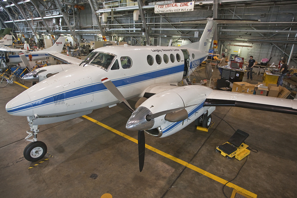
One of the instruments used in Operation IceBridge (OIB) is an airborne gravimeter operated through a collaboration between Lamont Doherty Earth Observatory of Columbia University and Sander Geophysics. Some people from other instrument teams call it a gravity meter, gravity, gravitometer, gravy meter, gravel meter, gravitron, or blue couch-like instrument. As operators of the gravimeter, we are referred to as graviteers, gravi-geeks or gravi-gods. This tells a lot about how mysterious and unknown this technology appears.

Let me summarize the basics of airborne gravity data acquisition for you.

But first, why is gravity data being acquired as part of OIB?

The earth’s gravity field is varying in space according to variations in topography and density distribution under the earth’s surface. Essentially, the greatest density contrast is between air (0.001 g/cc), water and ice (1.00 and 0.92 g/cc, respectively) and rocks (2.67 g/cc in average). Therefore, gravity data can be used for modelling the interface between these three elements. The ATM system (laser scanner) can locate the interface between air and whatever is underneath it with great accuracy. The MCoRDS system (ice penetrating radar) is successful at locating the interface underneath the ice. However, no radar system can “see” through water from the air. Hence, gravity data can help determine bathymetry beneath floating ice, either off shore or on shore (sub-glacial lakes). This in turn enables the creation of water circulation models and helps to predict melting of the ice from underneath. Also, airborne gravity data can contribute to increasing the accuracy and resolution of the Earth Gravitational Model (EGM), which is determined only with low resolution in remote locations such as the poles, being built mainly from data acquired with satellites.

Most people don’t know that it is possible to acquire accurate gravity data from a moving platform such as an aircraft. Due to the vibrations and accelerations experienced by the aircraft, it is definitively a challenge! There are four key elements that make this possible.

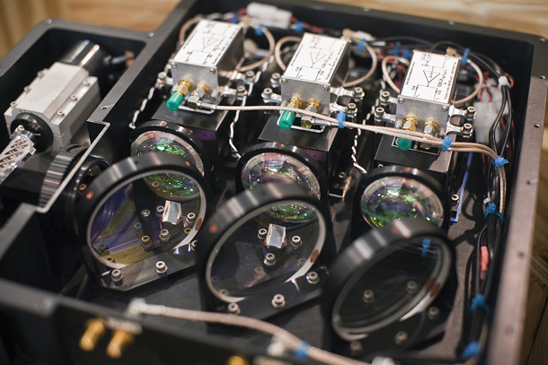
1- You must have very accurate acceleration sensors, called accelerometers.

2- You must keep these accelerometers as stable as possible, and oriented in a fixed direction. This is a job for gyroscopes coupled with a system of motors that keeps the accelerometers fixed in an inertial reference frame, independently of the attitude of the aircraft. This is why the system we use is called AIRGrav, which stands for Airborne Inertially Referenced Gravimeter. Damping is also necessary to reduce transmission of aircraft vibrations to the sensors. The internal temperature of the gravimeter also has to be kept very stable.

This is all good. However, the accelerations we are measuring this way are not only due to the earth’s gravity pull, but also (and mostly) due to the aircraft motion. And to correct for that:

3- You need very accurate GPS data, so that you can model the aircraft motion with great precision.

Despite these best efforts, noise remains, mostly from GPS inaccuracies and aircraft vibrations that can’t be detected by GPS, so:

4- You have to apply a low pass filter to the data, since the noise amplitude is greatest at high frequency.

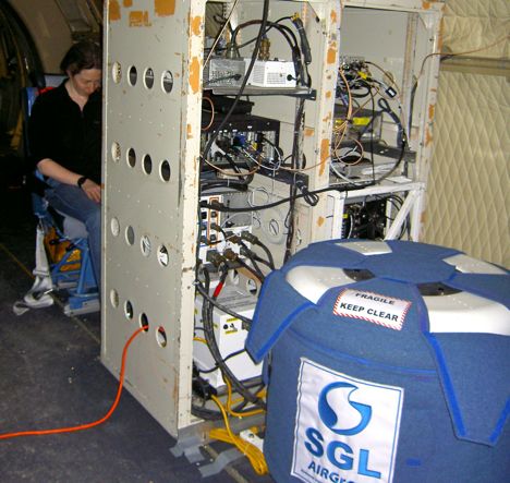
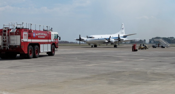
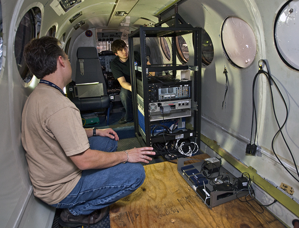
The AIRGrav system on-board the P-3 aircraft. Gravimeter (right), rack equipped with computers controlling the gravimeter and GPS receivers (center) and operator (left). Credit: Joël Dubé

Furthermore, a number of corrections have to be applied to the data before they can serve the scientific community. The corrections aim at removing vertical accelerations that have nothing to do with the density distribution at the earth’s sub-surface.

The Latitude correction removes the gravity component that is only dependent on latitude. That is the gravity value that would be observed if the earth was treated as a perfect, homogeneous, rotating ellipsoid. This value is also called the normal gravity. Since the earth is flatter at the poles, being at high latitude means you are closer to the earth’s mass center, hence the stronger gravity. Also, because of the earth’s rotation and the shorter distance to the spinning axis, a point close to the pole moves slower and this will add to gravity as well (less centrifugal force acting against earth’s pull).

Anything traveling in the same direction as the earth’s rotation (eastward), will experience a stronger centrifugal force thus a weaker gravity, and the other way around in the other direction. Traveling over a curved surface also reduces gravity no matter which direction is flown, similar to feeling lighter on a roller coaster as you come over the top of a hill. This is known as the Eötvös effect and is taken care of by the Eötvös correction. This correction is particularly important for measurements taken from an aircraft moving at 250-300 knots.

The Free Air correction simply accounts for the elevation at which a measurement is taken. The further you are from the earth’s center, the weaker the gravity.

To give you an idea of how small the gravity signal that we are interested in is with respect to other vertical accelerations that have to be removed, let’s look at the following profiles made from a real data set. All numbers are in mGals (1 m/s2 = 100,000 mGals), except for the terrain and flying height which are in meters.

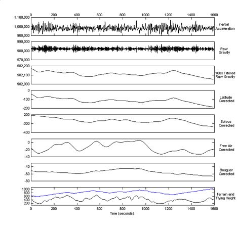
A visual summary of gravity corrections. Credit: Stefan Elieff

“Raw Gravity” in this diagram means that GPS accelerations (aircraft motions) have been removed from inertial accelerations. Notice the relative scales of the profiles, starting at 200,000 mGals, down to 20,000 mGals when aircraft motions are accounted for, down to 200 mGals after removing most of the high frequency noise, and ending at 50 mGals for Free Air corrected gravity. Free Air gravity is influenced by the air/water/ice/rock interfaces described earlier, and since OIB uses the gravity data to find the rock interface (the unknown), Free Air gravity is the final product. As a side note, for other types of gravity surveys, we usually want to correct for the terrain effect (the air/water/rock interfaces are known in these cases), so that we are left with the gravity influenced only by the variations of density within the rocks. This is called Bouguer gravity and is also shown in the figure.

Notice the inverse correspondence between flying height (last profile, in blue) and the profiles before the free air correction (going higher, further from the earth, decreases gravity), and the correspondence between terrain (last profile, in black) and the free air corrected data.

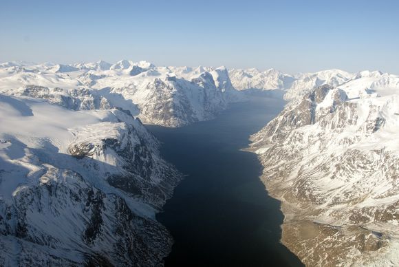
Now, let’s look at some data acquired during the current 2011 mission in western Greenland.

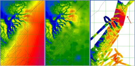
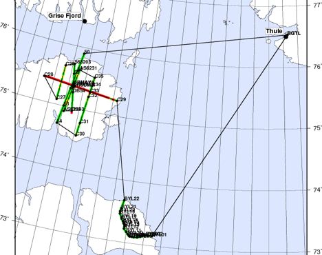
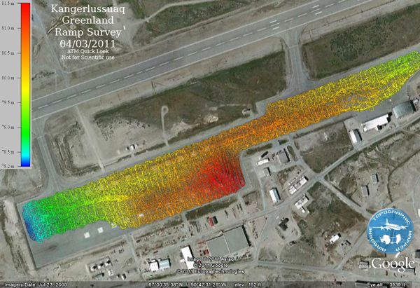
Ice elevation (left), rock elevation (middle) and Free Air gravity data (right). Greenland 2011 flight lines shown in black. Gravity data is preliminary and is not yet available for scientific analysis.

The left panel shows the elevation of the rocks, or of the ice where ice is present. It is as if the water has been drained from the ocean. The middle panel shows only the bedrock elevation, both ice and water being removed. The data is from ETOPO1, a global relief model covering the entire earth. The right panel shows the Free Air gravity acquired in the last few weeks. Most channels, called fjords, are well mapped by the gravity data. It is interesting to see that the gravity data infers the presence of a sub-glacial channel (shown by the red arrow) where no channel is mapped (yet?) on the bedrock map. The most likely reason for this is that this particular region has not been covered by previous ice radar surveys (there are huge portions of the Greenland ice sheet that remain unexplored). Note that the MCoRDS ice radar data acquired as part of the current campaign will improve the resolution in this area and will enable for a better comparison of both data sets in the future.

Advancing Ice Science from All Angles

From: Kathryn Hansen, NASA’s Earth Science News Team


On May 5, 2011, IceBridge surveyed the Devon Ice Cap (above) and two glaciers on Bylot Island (below). Credit: NASA/John Sonntag

Thule, Greenland — On May 5, 2011, Operation IceBridge completed its third and final flight in conjunction with an experiment operated by the European Space Agency (ESA).

The experiment, called CryoVEx, is a series of ground-based calibration sites for ESA’s ice-observing satellite, CryoSat-2. IceBridge flights over these calibration sites ultimately are expected to provide data to evaluate and improve remote-sensing measurements.

“The collaboration will also help us to jointly interpret measurements collected from the ground, air and space, advancing our understanding of ice sheets and sea ice, and their response to climate change,” said Michael Studinger, IceBridge project scientist.

The morning of May 5 started like most days in the field with IceBridge – with an early-morning weather brief. Poor weather afflicted most remaining science sites accessible by the P-3 that day, so IceBridge teams looked toward Canada. A phone call to researchers at Summit Camp on Canada’s Devon Ice Cap – the site of the final CryoVEx site – revealed good conditions.

In the Arctic, however, weather can turn on even the best-informed observations and predictions.

Summit Camp on Canada’s Devon Ice Cap is visible from the P-3, which overflew the ground-based calibration site on May 5, 2011. Credit: NASA/Digital Imaging Sensor

“We flew over the camp and the corner reflectors several times,” Studinger wrote in the mission’s situation report. “Conditions changed quickly. On the last flight we could barely see the camp.”

Still, the clouds parted long enough for the Airborne Topographic Mapper (ATM), a laser altimeter that measures surface elevation, to achieve good data from 75 percent of the area surveyed on the Devon Ice Cap.

Weather was more favorable south of Devon Island over Bylot Island, where the P-3 flew a first-time survey of two Bylot glaciers and collected good data over 90 percent of area surveyed. Credit: NASA/Michael Studinger

The campaign’s previous collaboration with CryoVEx included a flight on April 15 over sea ice, and on April 26 over the interior of the Greenland Ice Sheet.

“This has been a great collaboration between ESA and NASA for cryospheric and airborne science, and will no doubt lead to further joint activities in the future,” Studinger said.

The Long Wait

From: Lora Koenig, NASA’s Goddard Space Flight Center, Operation IceBridge Deputy Project Scientist

It arrived, finally it arrived! Yes, the new B200 windshield is here and currently being installed. You begin to realize how remote Kangerlussuaq, Greenland, is when you need something. In the United States you can overnight ship almost anything from Chicago style pizza to Memphis ribs to aircraft windows, but not here. Here, in Kangerlussuaq, the only way to get things this time of year is on one plane that arrives from Copenhagen, Denmark, Monday through Friday at 9:30 a.m. local time.

When the B200 windshield cracked on Monday the plane crew immediately ordered a new windshield to be sent from NASA Langley. It was shipped on Tuesday and arrived today. During the time that it took the windshield transit, the B200 plane crew took out the old windshield and prepped the plane for the new one.

I have learned a lot about aircraft windshields the past few days. For instance aircraft windshields are installed using a sealant (a glue to secure the windshield inside a bolted frame). Even though it has warmed up significantly since we first arrived, it’s just 27 F (-3 C) outside. That’s quite balmy compared to the -8 F (-22 C) temperatures of last week, but the windshield sealant needs temperatures around 77 F to cure. The aircraft is in a hanger but it is still too cold to cure quickly. The B200 crew spoke with some of the Air Greenland crew who lent us some Infrared (IR) heating lamps. The IR heating lamps will allow us to install the window and cut the curing time in half so we can get back in the air sooner.

Right now the window is being installed and sealant applied. Overnight, the window will sit under the IR lamps. On Saturday the plane will undergo a test flight with only the pilots onboard to ensure the aircraft is safe. If all goes well by Monday we will be back up and flying the B200, which carries a high-altitude laser altimeter called the Land Vegetation and Ice Sensor (LVIS).

In the meantime the LVIS instrument has been resting but Elvis sightings around Greenland have remained high.

The first Elvis sighting was Rob White (left) from the B200 crew, and the second Elvis sighting was Shane Wake (right), an LVIS instrument operator. 

Mission Mop Up

From: Kathryn Hansen, NASA’s Earth Science News Team / Cryosphere Outreach

April 8, 2011

Kangerlussuaq, Greenland — Today’s mission was a mix of the exciting and dull – from spectacular scenery over an ice cap, and up some glaciers and over Jakobshavn’s calving front, to the monotonous but scientifically important back-and-forth mapping of Russell glacier. It was essentially a “mop up” mission, combining targets from three separate flight plans.

We starting the day off flying over Sukkertoppen Isflade, our first ice cap of 2011! Flying over the blanket of ice, the scene abruptly ends as ice cascades down steep terrain into an open-water fjord that separates the ice cap from the Greenland Ice Sheet. Ice caps, while separate from the main ice sheet, are also undergoing changes and contribute to sea level rise.

An open-water fjord separates the Sukkertoppen ice cap from the Greenland Ice Sheet. Credit: NASA/Michael Studinger

Continuing south, we flew along several glaciers starting with Taserssuak (not thinning) and later on over Kangiatanunatasermia (thinning). The difference is interesting, as both glaciers are fed by the same fjord system. Scientists want to keep watch over these regions to continue to see how the change is changing.

We flew four glaciers fed by the Nuuk flord system including this glacier with a colorful name, Akugdlerssupsermia. Credit: NASA/Robbie Russell

After hitting some clouds as expected from the morning’s weather brief, we headed back north and reflew the center flow line of Jakobshavn — always spectacular — before flying over Illulisat Isfjord, which was surprisingly free of ice. The reason for the ice-free conditions was unknown to scientists onboard. There could have been fewer calving events, warmer water, or wind patterns that pushed ice out of the area.

“Half of the Illulisat Isfjord was open water with several fishing boats in the area, something I have never seen before,” said Michael Studinger, the mission’s project scientist.

A camera mounted on the belly of the aircraft captured this image of a fishing boat (top) in the Illulisat flord, which was mostly open water with a few visible patches of ice. Credit: NASA/DMS team

Next it was on to Russell Glacier, just outside of our home base, Kangerlussuaq. Back and forth, this was a true “moving the lawn” pattern. I may have even taken a brief nap. But to scientists, this mapping is critical. A radar instrument onboard will get a good look at what’s below all that ice and help scientists better understand how the bedrock influences the flow of glaciers.

Battling the Arctic Chill

From: Kathryn Hansen, NASA’s Earth Science News Team/Cryosphere Outreach

April 6, 2011

Kangerlussuaq, Greenland — It may seem obvious, but the Arctic is cold. I was surprised to arrive in Kangerlussuaq, Greenland, to see the hills and streets covered with snow and temperatures that make you second-guess the wisdom of leaving any skin exposed.

In 2010, the Kangerlussuaq leg of Operation IceBridge began about a month later, in May. What a difference a month makes. The hills were snow-free, flowers beginning to bloom, days were long, and the river rushed to break up the last chunks of winter ice. On down days, crew and science teams hiked, biked and went fossil hunting. Now we mostly stick to the warm indoors. Most of us, however, are willing to brave the cold and dwindling hours of darkness to catch a spectacular show of the northern lights.


This time lapse of the northern lights consists of 30-second exposures spanning just over an hour. We took turns behind the camera, running inside every 15 minutes to quickly warm up. Credit: NASA/Jefferson Beck

It turns out that the aircraft also battles the cold. On April 5, we planned to fly the mission’s first science flight from Kangerlussuaq to collect data over Jakobshavn — Greenland’s fastest moving glacier. At 6 a.m. it was just -11 F. The coffee pot onboard froze and fractured.

Shortly after take off, the cold temperatures resulted in a mechanical issue on the aircraft that forced an early return to Kangerlussuaq, Greenland. The P-3’s adept aircrew was quick to diagnose and resolve the issue.

John Doyle, a P-3 flight mechanic, is on the aircraft early and prepared for the cold. Credit: NASA/Kathryn Hansen

On April 6, crew started the day extra early at 5:30 a.m. when the temperature measured in even chillier at -18 F. Additional heating for an extended period prior to flight led to a successful first flight from Kangerlussuaq. And what a spectacular, clear flight.

The DMS, a downward looking camera system, captured this shot of Jakobshavn’s calving front. Credit: NASA/DMS team

Instrument teams onboard the P-3 also battle with the effects of temperature. Scientists with the laser altimeter use hair dryers to warm up the instrument, but too hot is also problematic. Scientists working with the radar instruments prefer the cooler time of year before melt ponds appear on the ice, complicating the way light reflects from the surface.

Having overcome challenges posed by the cold, we’re looking forward to a long series of land ice flights over Greenland. There’s word among the crew that the new coffee pot should arrive in a few weeks, in time for IceBridge’s return to Thule. Thanks to the P-3 crew for what might be the best cup of Joe in Greenland!

In the absence of coffee pot, P-3 crew construct a makeshift filter out of a water bottle. Credit: NASA/Kathryn Hansen

A Five-Hour Survey

From: Kathryn Hansen, NASA Earth Science News Team / Cryosphere Outreach

April 3, 2011


Colors show elevation differences across the airport’s ramp in Kangerlussuaq, Greenland. The map is used to calibrate airborne instruments. Credit: NASA/ATM team

Kangerlussuaq, Greenland — During the last IceBridge campaign, based in Punta Areans, Chile, we described a three-hour ramp survey. Scientists drove a truck with a GPS antenna affixed to the roof to map the precise elevation of the airport’s entire ramp — the pavement next to the runway where the aircraft spends each night. The ramp map helps researchers calibrate science instruments on the aircraft.

Here in Greenland, at Kangerlussuaq International Airport, the same activity on Saturday, March 3, would turn into a five-hour survey.

“This has to be the biggest ramp in the world,” said Kyle Krabill who drove the car, bringing me along as the unsuspecting passenger.

The task started that morning after idling for an hour on the ramp to calibrate the GPS. Then, we rolled off at a whopping 15 miles per hour, windows rolled down and 80’s Danish music blaring. Back … and forth … and back … and forth … we traced around the perimeter of the ramp and then inward, as if we were mowing a lawn of pavement.


A time lapse shows one hour of four-hour-long ramp survey. Video credit: NASA/Jefferson Beck

“See how easy it is to be a scientist?” Krabill joked. But it turns out that driving the car is just the beginning.

Krabill is part of the team that runs the Airborne Topographic Mapper (ATM), an instrument flying with IceBridge. ATM pulses laser light in circular scans on the ground. The pulses reflect back to the aircraft and are converted into elevation maps of the ice surface.

Toward the end of each flight, ATM laser elevation data are also collected during a pass over the ramp. Putting the data all together (including the dizzying ground-based ramp survey), and knowing the precise location of the aircraft (via a technique called “differential GPS”) scientists can decipher and eliminate some of the inherent error that comes with flying a laser scanner, such as errors in range — the physical distance to the ground — and in the team’s knowledge of the way in which the scanner is mounted in the aircraft.

“Differential GPS is fundamental to what we do,” said John Sonntag, ATM senior scientist. “It’s tremendously powerful, taking position error down from about 10 meters to 10 centimeters or better — a huge improvement.”

P-3 Back in Service

April 2, 2011

Kangerlussuaq, Greenland — The P-3 is ready to return to IceBridge just 30 hours after the aircraft’s prop valve failed on Friday, April 1. Here we list highlights from the tremendous effort by aircraft crew who were responsible for the speedy return to flight.

P-3 crewmen John Doyle and Brian Yates work on engine #2. Credit: NASA/Jim Yungel


Friday morning:

1. From Kangerlussuaq, Greenland, get permission to ferry the aircraft to its home in Wallops Island, Va.

2. Line up customs at Dover Air Base

3. File a flight plan

4. Fuel the aircraft

Friday night:

5. Remove the propeller on engine #2

Saturday morning:

6. Replace the P-3 propeller valve

7. On the ramp, let the aircraft’s engine run

8. Functional checkout flight (successful!)

Sunday:

9. Take a much-deserved mandatory hard down day in Wallops Island, Va.

Monday:

10. The P-3 is scheduled to depart Wallops at 7 a.m. EDT and arrive in Kangerlussuaq at 4:30 p.m. local time, ready for a possible flight on Tuesday!

Engine run up under way on the ramp at Wallops. Credit: NASA/Jim Yungel

LVIS is in the Building

From: Kristyn Ecochard, NASA’s Langley Research Center

Crewmembers are busy getting the B-200 King Air at NASA’s Langley Research Center in Hampton, Va. ready for its first flight with Operation IceBridge.

The King Air will be carrying the Land Vegetation and Ice Sensor (LVIS) onboard for several weeks of science flights over the Arctic. LVIS is an instrument from NASA’s Goddard Space Flight Center in Greenbelt, Md.

Engineers are uploading the instrument and other science equipment in preparation for a scheduled departure date of April 13.

IceBridge teams are already in Greenland conducting science flights onboard the P-3B based out of NASA’s Wallops Flight Facility in Wallops Island, Va.

The B-200 King Air at NASA’s Langley Research Center is a small plane that can get up to 35,000 feet. Credit:NASA/Sean Smith


The King Air will only carry one instrument on its science flights over the Arctic: the Land Vegetation and Ice Sensor (LVIS) operated by NASA Goddard Space Flight Center’s David Rabine and Shane Wake. Credit:NASA/Sean Smith


NASA Goddard Space Flight Center’s Land Vegetation and Ice Sensor (LVIS) will map large areas of sea ice and glacier zones. Credit: NASA/Sean Smith

Keeping Us On Track

From: John Sonntag, ATM Senior Scientist and IceBridge Instrument Team Lead

Thule, Greenland — One of the many unusual aspects of flying with NASA’s Operation IceBridge (OIB) is that we fly very, very precisely. Getting the airplane where we want it to be, when we want it to be there is important for a variety of reasons. At its most basic, however, precise flying is necessary to match the limited footprint of our remote-sensing instruments with the target they are measuring. This target might be a spacecraft ground track, the centerline of the fastest-moving channel of a steep, sinuous glacier, or even a research camp established on a drifting ice floe.

Our pilots are outstanding professionals and the precise flying is primarily their doing. But to help them do it, OIB leverages NASA’s multi-decade investment in operations of the Airborne Topographic Mapper (ATM), a scanning lidar and key instrument of OIB. The ATM project, which is my own home team and where I learned most of what I know about airborne science, long ago addressed the need to fly a remote-sensing aircraft very accurately over regions with no fixed landmarks. The key, not surprisingly, is the Global Positioning System, or GPS. GPS, of course, gives us nearly continuous updates of our position with an accuracy of just a few meters. But using this knowledge effectively, especially at 250 knots, is a little tricky.

So the ATM team developed, and continues to modernize, a suite of software and hardware tools to effectively use GPS to help pilots steer an airplane very accurately, and even to steer the airplane directly. In their current form these tools are called “SOXMap and SOXCDI”.

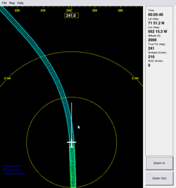
SOXMap is really just a “moving map” system, at heart not unlike the ones in consumer GPS units used in cars or for hiking, but simpler and highly specialized for remote sensing applications. SOXMap displays the aircraft’s current position and orientation relative to a science target, such as the sinuous centerline of a glacier (see the SOXMap illustration, left). It also displays the measurement swath being collected by a science instrument such as the ATM, drawn to scale. This display is piped to the pilots up front, using little tablet computers with very sharp, bright displays, which are mounted right on the control yoke. Our pilots use this information, which is continuously updated, to steer the aircraft and its sensor swath right where we want it. Some of our OIB pilots refer to SOXMap as “the Pac Man display”, in reference to the old video game where the player guides a little mouth around a screen chewing up dots. The beauty of SOXMap is its versatility. Our bread-and-butter use for it with OIB is to follow sinuous glacier centerlines with any degree of curvature, but SOXMap is also useful for area-mapping applications, or really any targeted flying.

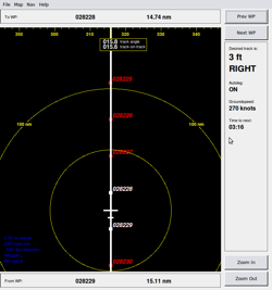
Even cooler than SOXMap is its sibling, “SOXCDI”. SOXCDI (image right) incorporates a moving map display similar to the one in SOXMap, but unlike SOXMap, SOXCDI can actually steer the airplane automatically! It is designed for cases where we fly long straight lines, such as grid lines or satellite ground tracks. We can do the same thing successfully using only SOXMap, but for long straight lines this demands lengthy periods of concentration from our pilots and can be extremely tedious for them. So SOXCDI continuously compares the current position of the aircraft to a desired straight-line track connecting a pair of waypoints (for any navigation geeks who might be reading along, the straight line is actually a great circle, and I plan to add a selectable rhumb line option as well). Doing a little math with that comparison, we always know how far we are from the desired track and whether we are right or left of it.

But how do we use this information to steer the aircraft automatically? Here is where things get extremely cool. It turns out that most large airplanes have what is called an “instrument landing system”, or ILS. The ILS is really just a radio receiver that is designed to listen to a simple pair of audible tones being broadcast from an airport runway, each tone angled slightly away from each side of the centerline. This allows them to land in bad weather when the runway isn’t immediately visible. If the ILS radio “hears” more of one of the tones than the other, it directs the pilot, actually the autopilot in our case, toward the “quieter” tone until the two tones are equal. When they are equal, the airplane is centered on the runway, right where it should be.

Can you guess where we’re going here? SOXCDI simply mimics an ILS signal, which we pipe into the aircraft’s autopilot. And it’s pretty simple, really. If we’re left of track, we generate more of the “left” tone than the “right” tone, and vice versa. The airplane’s autopilot does the rest. The tricky part comes in calculating how much of each tone we generate given how far right or left of track we are, but those are just details. The point is, the system is simple because we just piggyback on existing technology – the ILS. And though our software certainly has some complexity, the hardware is almost breathtakingly simple. We run the SOXCDI (and SOXMap) programs on very basic, run-of-the-mill computers – that 8-year-old laptop you tossed in the closet during the previous presidential administration would probably work fine once we installed our software on it. The tones are generated by the sound card built in to every modern computer has built in. We literally just plug a cable into the headphone jack of the computer, and plug the other end into a standard piece of lab equipment called a “function generator.” The function generator just takes the two tones and turns them into a radio signal, which we then pipe via another cable into the airplane’s ILS. And that’s it. You might not be familiar with a function generator, but to give you an idea what a basic piece of lab equipment it is, we recently bought one for just about $1,000, about what a basic laptop costs.

Once it’s all set up, SOXCDI generally keeps the airplane within just a few meters of where we want it to be, and can do it literally all day long. It does this, in essence, by “singing” a two-note chord to the airplane, the relative volumes of the two notes determining the steering correction. And it works equally well with both of NASA’s workhorse OIB airplanes – the P-3 turboprop and the DC-8 jet. And that points to another strength of the SOXCDI design. Because it mimics standard ILS signals, it should work with any ILS-equipped airplane.

If I sound enthusiastic about our precise navigation systems, well, I am. I am the developer of SOXMap and the co-developer of SOXCDI with my colleague Rob Russell, and I’m very proud of their role as a key enabling technology for IceBridge. They are also just about the most fun projects I’ve ever taken on at work, a perfect task for an at-heart aerospace tinkerer like me. But Rob and I can’t claim all the credit, or even most of it. We built SOXCDI and SOXMap on ideas originally conceived and developed by our colleagues Wayne Wright (SOXCDI predecessors), and Richard Mitchell and Bob Swift (SOXMAP predecessors), respectively.

And finally, what about those names? Well, the original implementation of the moving map concept with the sensor swath drawn to scale, way back in the 90s, was called XMAP. So in homage to that, I originally called my implementation “Son Of XMAP”, which became SOXMap. Later when we developed SOXCDI, we essentially merged elements of SOXMap and and older system called CDI (for Course Deviation Indicator), yielding SOXCDI.