By George Hale, IceBridge Science Outreach Coordinator, NASA Goddard Space Flight Center
An IceBridge field campaign is the culmination of months of planning and preparation. At January’s science team meeting, scientists focused the campaign’s goals and provided mission planners the details needed to finalize flight plans. With these final details ironed out the next step was to start preparing the tools of the trade, IceBridge’s aircraft and instruments. For the past several days, instrument teams and aircraft technicians at NASA’s Wallops Flight Facility in Wallops Island, Va., have been getting the P-3B ready for the 2013 Arctic campaign, which is scheduled to have its first science flight on Mar. 20.
Operation IceBridge is but one of several missions to use NASA’s P-3B airborne laboratory. After each mission, this aircraft returns to its home base at Wallops where it undergoes repairs and routine scheduled maintenance needed to keep it flying at peak efficiency and where science instruments are swapped out. This rotation of airborne science missions keeps the Wallops aircraft team busy, preparing between three and five missions per year. “Sometimes it’s more and sometimes it’s less,” said P-3B flight engineer Brian Yates. “We’re working on some relatively large projects, so we have five this year.”

After the aircraft’s maintenance is complete and the previous mission’s equipment has been removed, the IceBridge team starts installing the mission’s suite of science instruments. This process can be generally divided into a few portions: installing the instrument and the equipment needed to control it and collect data, testing the individual instruments and checking to make sure the aircraft and instrument suite work together as they should.
The first step is installing the components that gather the data, such as cameras, radar arrays and laser transceivers. The Airborne Topographic Mapper (ATM) laser and Digital Mapping System (DMS) cameras are installed in bays on the underside of the aircraft. Each of these instruments looks down through windows in the plane’s belly. The Multichannel Coherent Radar Depth Sounder (MCoRDS) antenna is attached to the underside of the aircraft. Previously this has included antennas under the wings, but IceBridge is flying with a trimmed down MCoRDS instrument with an array beneath the P-3B’s fuselage.Additional radar instruments like the accumulation and snow radars and Ku-band radar altimeter are also installed at this time.
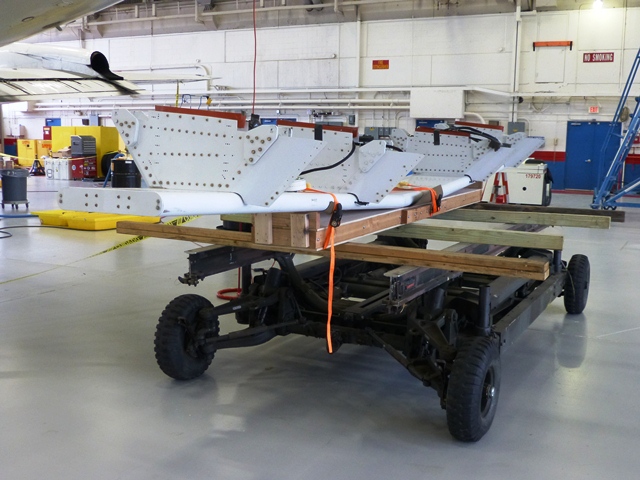
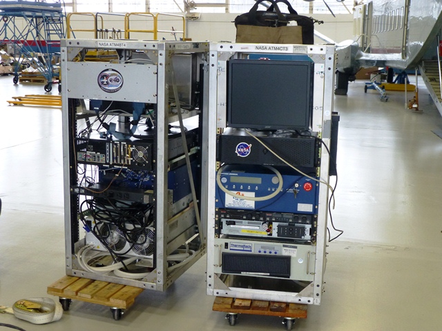
While this hardware was being installed on the plane, other members of the instrument team put together all of the hardware needed to operate the instruments in metal racks that are then securely bolted to the floor of the plane. Making sure everything is securely fastened is crucial because of the often turbulent nature of low-altitude polar survey flights.
Once everything is in place and secured the next step is to make sure the instruments work properly. This means rounds of testing both on the ground and in the air. Ground testing involves checking instrument connections and alignment. “We’ll check on the camera to make sure it’s seeing through the window ok and not catching the edge,” said DMS field engineer Dennis Gearhart.
Everything being used in this IceBridge campaign has flown before, but it’s important to make sure the instruments are working properly.”We want to make sure things work as well as they did when they were put into storage,” said ATM program manager James Yungel. To do this, the ATM team will bounce the laser off a ground target 500 feet away.

The real test of all this work comes with the mission’s check flights on Mar. 13 and 14. The first flight, known as an engineering check flight is carried out with flight crew only and is to ensure that everything is properly installed and secured. Scientists and instrument operators participate in the second flight, where instruments are powered on and tested. “The check flights are a final arbiter,” said Yungel.
This year’s IceBridge Arctic campaign will run from Mar. 18 through May 3. The P-3B will operate out of airfields in Thule and Kangerlussuaq, Greenland, and Fairbanks, Alaska.
NASA Goddard Hosts IceBridge Science Team Meeting
By George Hale, Science Outreach Coordinator, NASA Goddard Space Flight Center
Large scientific missions like IceBridge take continual planning to keep running. In addition to regular telephone and email collaboration, IceBridge researchers meet in person twice a year to discuss the mission’s science aims, results and plans for future campaigns. The first of 2013’s IceBridge science team meetings and the annual meeting of the Program for Arctic Regional Climate Assessment (PARCA) took place at NASA’s Goddard Space Flight Center in Greenbelt, Md., Jan. 29–31.
The IceBridge science team is a group of polar scientists from a variety of institutions and serves multiple functions. The largest of these functions is guiding the mission toward meeting its science requirements.”The team provides general guidance and advice,” said IceBridge project scientist Michael Studinger. “They look at how far down the road we are to meeting our level one science requirements.”
The science team meeting was joined by the annual meeting of PARCA, a NASA initiated program started in 1995 to understand changes to the Greenland Ice Sheet. This was to be accomplished through periodic airborne surveys, satellite remote sensing and surface-based research. Starting in 2009, PARCA’s annual meeting has been scheduled to coincide with IceBridge’s science team meeting. “Originally PARCA was a Greenland field campaign planning meeting,” said NASA scientist Charles Webb. “Having the meetings together logically makes sense.”
")
NASA scientist Bryan Blair gives a presentation on the future of the Land Vegetation and Ice Sensor (LVIS). Credit: NASA / Jefferson Beck
Presentation topics at both meetings ranged from the use of IceBridge data in seasonal sea ice forecasts to the use of radar to image layers in ice sheets to new algorithms for mapping bedrock beneath the ice.Other presentations included status updates for instruments like the Airborne Topographic Mapper (ATM) and Land, Vegetation and Ice Sensor (LVIS) and a look ahead at NASA’s next-generation polar monitoring satellite, ICESat-2.
The PARCA meeting started on Jan. 29 with sessions on newresearch and novel ways to work with IceBridge and other cryospheric data. Participantsclosed out a busy day with a remembrance of cryospheric scientist SeymourLaxon, whose unexpected death earlier in the month shocked the polar sciencecommunity, and a poster session and dinner at Goddard’s recreation center.
PARCA sessions finished up on the morning of Jan. 30, covering integrating IceBridge data, radar mapping of ice sheets and next steps in ice sheet physics. After lunch, the IceBridge science team meeting started, with breakout sessions by the sea ice and land ice science teams. In these sessions,science team members discussed research and plans for the upcoming IceBridge Arctic campaign and beyond, including collaborations with various other groups outside of NASA. Later in the day, ATM senior scientist John Sonntag presented planned flight lines for the 2013 Arctic campaign and invited comments on suggestions for ways the lines can better meet IceBridge’s science goals.

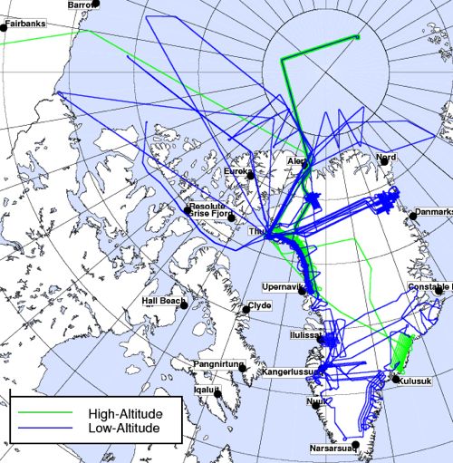
ATM senior scientist John Sonntag shows proposed flight plans for 2013 Arctic campaign. Credit: NASA / Jefferson Beck
The last day of the IceBridge science team meeting saw more sessions on IceBridge science, data and future plans. Included in the sesessions were talks about new instruments like a version of LVIS soon to be tested on NASA’s Global Hawk, status updates on ICESat-2 and a final discussion of proposed flight lines for the IceBridge Arctic campaign, where flight plans were assigned priorities and finalized. This year, IceBridge science team member Robin Bell from Lamont-Doherty Earth Observatory of Columbia University came up with a new and hands-on way to improve this process. Bell set up three tables representing high, medium and low priorities, onto which printed copies of flight plans were sorted. “This gave us a more visual and intuitive feel for how the flight lines fit together,” said Sonntag. “It was a good way to get flight priorities straightened out.”
This sort of discussion, where scientists hash out details on research goals, priorities and methodologies is at the heart of not only IceBridge, but scientific work in general. “The research landscape is constantly evolving, so you have to rethink how you approach problems and organize the community once in a while,” said Studinger. “You need constant evaluation and discussion of ideas and results.”

Science team members sort through printed copies of proposed flight lines. Credit: NASA / Jefferson Beck
Operation IceBridge Featured in EOS
By George Hale, IceBridge Science Outreach Coordinator, NASA Goddard Space Flight Center
The new quick look sea ice data product released by NASA’s Operation IceBridge was the subject of a cover story in the Jan. 22 issue of the American Geophysical Union publication EOS. The article discusses the sea ice data product created by IceBridge scientists during the 2012 Arctic campaign last April and how these datasets provide new ways for researchers to measure Arctic sea ice.

EOS article:
http://onlinelibrary.wiley.com/doi/10.1002/2013EO040001/abstract
For more about IceBridge’s quick-look sea ice product and its use in seasonal forecasts, visit:
https://www.nasa.gov/mission_pages/icebridge/news/spr12/arctic-seaice.html
https://www.nasa.gov/topics/earth/features/seaice-forecasting.html
Q&A: Michael Studinger
By Maria-Jose Viñas, Cryospheric Sciences Laboratory Outreach Coordinator, NASA Goddard Space Flight Center
Michael Studinger is Operation IceBridge’s project scientist. He trained as a geophysicist in Germany, his home country, before moving to the U.S. to take a position at the Lamont-Doherty Earth Observatory and then transferring to NASA Goddard Space Flight Center in 2010. Studinger has been studying polar regions for 18 years, expanding his initial focus on the geology and tectonics of the Antarctic continent to the overall dynamic of polar ice sheets.

Operation IceBridge Project Scientist Michael Studinger. Credit: Jefferson Beck / NASA
Studinger recently returned from Greenland, where he was leading Operation IceBridge’s 2012 Arctic campaign.
This was IceBridge’s fourth Arctic campaign. How different was it from previous years?
We flew more than last year: During the 75 days we were there, we only had to cancel a single flight because of weather, something I’ve never seen before. Regarding sea ice, we have expanded coverage in terms of area. For the first time we went to the Chukchi and Beaufort Seas to collect data there. But the biggest change this year is that we published a new data product that we had to deliver to the National Snow and Ice Data Center before we even returned from the field. This product is being used by modelers and other scientists to make a better prediction of the annual sea ice minimum in the summer. We can now feed ice thickness measurements from March and early April into these predictions and see how they improve them.
What are the benefits of improving Arctic sea ice minimum predictions?
There seems to be enough people who have an interest in finding out how thick or thin the sea ice will be. People who live in the Arctic and shipping companies…they want to know, they want to prepare. It’s like long-range weather forecast: People who grow crops would like to know if they’re going to get a wet season or a dry season.
Also, it’s a relatively short-term prediction, so we’ll soon find out if the models are working or not. It helps building better models because you can compare the results to the reality in a few months.
This Arctic campaign, you teamed up with CryoVEx, ESA’s calibration and validation campaign for the CryoSat-2 satellite. How did it go?
We did two coordinated flights with them. We were in Thule, Greenland, and they were in Alert, Canada. We both took off at the same time and made sure we were over the same point in the Arctic Ocean with CryoSat-2 flying overhead. It was quite a bit of a coordination effort. We measured the same spot along the satellite track within a few hours. The CryoVEx team has instruments similar to ours, but also some that we don’t have. IceBridge has unique instrument suite for sea ice that includes the world’s only airborne snow radar. By combining all the data from all the instruments, we can learn a lot about what each instrument is seeing and what CryoSat-2 is actually measuring over sea ice.
How’s your average Arctic campaign?
We start in Thule because we want to get the sea ice flights out of the way early on, as long as it’s cold over the Arctic Ocean. It’s still fairly dark there, that far north [Thule is 750 miles north of the Arctic Circle]. We have just enough light in the second half of March to fly the sea ice missions, during the first three weeks of the campaign. Then we go down to central Greenland while it’s still cold there and start doing ice sheet flights, for three or four weeks. Then we go back to Thule because it’s getting too warm in southern Greenland, and we finish the ice sheet flights in the northern half.
Can you describe your daily routine while in Greenland?
We get up at 5 a.m. In Kangerlussuaq, we try to be in the air at 8:30, and in Thule we try to be flying at 8, when the airport opens. Eight hours later, we land. After that, we have a science meeting where we talk about how the flight went and the plan for the following day. Then we eat dinner, check email, look at data… all that before we go to bed and do it all over again the next day.
How do Arctic and Antarctic campaigns differ?
We use different aircraft: a P-3B for the Arctic and a DC-8 for Antarctica. In Greenland, when we fly out of Kangerlussuaq or Thule, we start collecting data pretty much right away, except for the sea ice missions. In Antarctica, we “commute” from Punta Arenas in southern Chile, which takes a few hours. Then we can only collect data for a few hours before we go back home to Punta Arenas. Typically, in the DC-8 we fly for 11 to 11.5 hours, much longer than the about 8 hours of flight with the P-3.
We actually fly more instruments on the P-3: the accumulation radar and the magnetometer (which is much easier to install on the P-3 than on the DC-8). We don’t really have the room in the fuselage to mount the accumulation radar antennas and there’s not really much of a need to use it in Antarctica. The snow accumulation in Greenland is higher. We can actually see annual layers with the accumulation radar but it’d be far more difficult in Antarctica because less snow falls there.
Personally, do you prefer one campaign to the other?
No, they’re just different. It’s a different airplane: the DC-8 is much more comfortable, less noisy. You don’t have the vibration of the P-3, so you can actually get a lot of work done on the transit flights. But the flights are very long.
And scientifically, is one campaign more interesting than the other?
Not for me. Most of my work I’ve done in Antarctica, but I’m getting more and more interested in what Greenland has to tell us. If you look at the two biggest glaciers we study, Jakobshavn Isbrae in Greenland and Pine Island Glacier in Antarctica, the kind of mechanism through which both glaciers are losing ice is similar — warm ocean water is melting the ice from underneath. So we’re studying similar processes. Antarctica is far more challenging to get there and collect data, but from a scientific point we need to do both, otherwise we’re missing part of the picture.
What’s the 2012 Antarctic campaign going to look like?
It’s going to be shorter for a number of reasons, mostly because the aircraft has already been committed for an international multi-aircraft experiment in Thailand, and it’s also committed afterward. We’ll try to fly as much as we can, we’ll be using two aircraft: a G-V from the National Science Foundation, flying at high altitude, and NASA’s DC-8 flying low.
What will the future bring for IceBridge?
The plan is we will start using unmanned aerial vehicles and we’ll probably be doing it mostly over sea ice in the Arctic Ocean, but we don’t know the details yet. We will be doing some test flights over the Arctic Ocean later this year with the Global Hawk, either with the radar or laser altimeter onboard. I don’t think we can replace manned aircraft completely over the course of IceBridge.
After ICESat-2 launches, will IceBridge continue to some extent?
There will always be airborne campaigns to some degree, because there are some datasets that we can only collect from planes, and we will also need to calibrate and validate the satellite data. We need a variety of different scales, wavelengths, different types of measurements in order to really answer the science questions that we have, such as what is the contribution of Greenland to sea level rise in the next 20 or 30 years. For example, if we only have ICESat-2 collecting measurements of how the surface elevation is changing, we’ll know a lot, but we’ll never be able to answer with certainty what is causing these changes. It’s almost like you’re taking the pulse of a patient; you’re only looking at the symptoms of the illness without understanding what’s causing it. In order to find out why the ice sheet is changing its surface, we need to understand what’s beneath the ice sheet because that’s what’s driving a lot of the dynamic changes. And those are datasets that you can’t collect from space, you need an airplane to go in there and get the greater picture of what’s below there and other things, like snow accumulation, which can be done much better from airplane. It’s not a single satellite that will provide us the answer, not a single airborne measurement – it all has to come together.
A Spanish version of this post is available on National Public Radio’s Science Friday blog.
An Uncommon Routine
From: Michael Studinger, IceBridge project scientist, Goddard Earth Sciences and Technology Center at the University of Maryland, Baltimore County
Thule Air Base, Greenland — The IceBridge team arrived in Thule last week and the campaign is off to a good start. We flew four out of five days last week and accomplished three sea ice missions including an underflight of the European Space Agency’s CryoSat-2 satellite over the Arctic Ocean. After a week here in Thule, we are settled in and our operations have become routine.
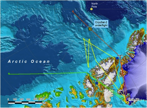
Operation IceBridge accomplished three science missions during the first week, including an underflight of ESA’s CryoSat-2 over the Arctic Ocean just 120 miles from the North Pole. Credit: NASA
A typical IceBridge day in Thule Greenland starts at 5 a.m. when my alarm clock goes off. I start downloading satellite images to get an idea which missions may be possible to fly before I go to breakfast at 5:45 a.m. At 6:15 a.m., the pilot in command, mission manager, John Sonntag and myself meet at Base Ops to get a weather brief for the day.
The three meteorologists at Thule Air Base have known us for years and do an excellent job in providing us with a very detailed and specialized weather brief that we require for decision making. The demands for research flights are different from everyday air travel, and the polar environment poses great challenges in terms forecasting the weather. There is not a single weather station within hundreds of miles of our survey area that we could use to get a weather observation or that would provide observational data as input into a forecast model. Instead, we depend on satellite images that are several hours old. Visible images are dark for any area west of us. It requires experience and skill to interpret the forecast products for our purpose.
A few days ago, a model transect along our flight path showed dense cloud cover along the entire mission profile at 500 meters flight elevation calling for a no-fly day. We spent time with the meteorologists to understand the weather situation and decided to fly, despite the grim looking forecast. It was the right decision. The cloud layer depicted by the forecast model turned out to be a thin layer of haze that did not pose any difficulties for our laser and digital imagery sensors.
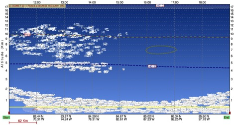
The weather forecast is shown along a survey line for a P-3 science mission. The forecast predicts dense cloud cover at the flight elevation (500 m), but after carefully studying the weather situation, we decided to fly. Credit: NASA
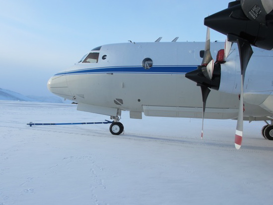
Between 6:30-6:45 a.m. we make a go/no-go decision. If we fly, the aircraft gets pushed out of the hangar and the fuel truck arrives. We need to collect one hour of static GPS data on the ground to calculate high-precision trajectory data from our flights. At 7:30 a.m. the door of the aircraft closes and we taxi to the runway to be ready for an 8 a.m. takeoff as soon as the tower opens.
We typically transit to the survey area north of Thule and then descend to 1,500 feet were we start collecting data. It’s still early in the season, which means missions west of Thule are flown in near-constant twilight, with the sun following us as we go west. When we turn around the western end of the line and fly back east, it immediately start getting lighter with every minute of the flight.
During the flight the operators monitor their instruments and make sure we collect high-quality data. Occasionally, adjustments need to be made to ensure the instruments keep working.
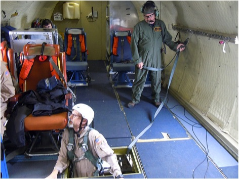
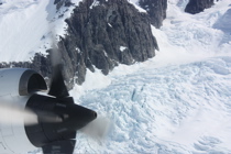
In-flight adjustments are often necessary to keep the instruments working and collecting high-quality data. Adjustments often require work below the deck to access the instrument sensors in the belly of the P-3. Credit: NASA/Michael Studinger
At 3:45 p.m. we typically land to leave enough time for a 1-hour post-calibration with the aircraft outside. By 5 p.m. the aircraft is rolled back inside the hanger and doors close for the night.
John Sonntag and myself quickly stop by Base Ops for another weather brief to see what’s in the mix for the next day. At 5:30 p.m. we have a science meeting where we discuss plans for the next day and talk about issues that are worth sharing with others. After the meeting, most people go straight to dinner followed by a late evening spent backing up data and processing data.
At 5 a.m. the next morning we start again.
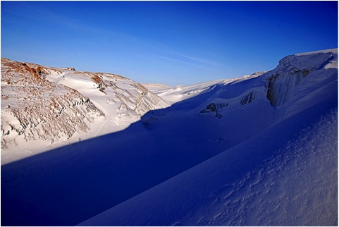
A lateral moraine can be seen at the margin of the Greenland Ice Sheet near Thule Air Base. Credit: NASA/Michael Studinger
Welcome to the 2011 Arctic Campaign
From: Kathryn Hansen, NASA’s Earth Science News Team/Cryosphere Outreach Specialist
On March 14, NASA’s P-3B landed in Thule, Greenland, for the start of the Arctic 2011 campaign of Operation IceBridge. Credit: NASA/Jim Yungel
On March 14, NASA’s P-3B aircraft landed in Thule, Greenland, where it will be based for the first leg of the Arctic 2011 campaign of Operation IceBridge. It’s our third annual campaign over the frozen north, ensuring the continuity of ice elevation measurements that scientists use to monitor change. This year, IceBridge is bigger than ever before and delving into new areas of exploration. Read more about the Arctic 2011 campaign and watch the video here.
Follow this blog throughout the 10-week campaign to read about the mission from the perspective of the scientists and crew on the ground (and in the air) who make the mission possible. They will give a behind-the-scenes account of individual flights and daily life in the field. They will share pictures and video from the sky and ground. And they will discuss the science questions being probed by the array of instruments onboard the flying laboratories. Welcome aboard!

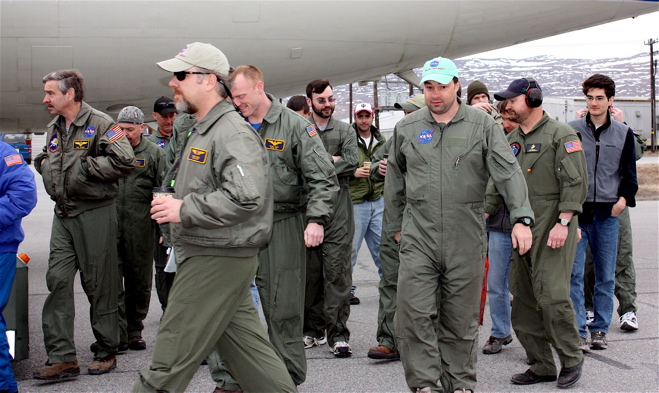
Mission participants chat inside the P-3B during transit on March 14 from NASA’s Wallops Flight Facility in Wallops Island, Va., to the mission’s base in Thule, Greenland. Credit: NASA/Jim Yungel
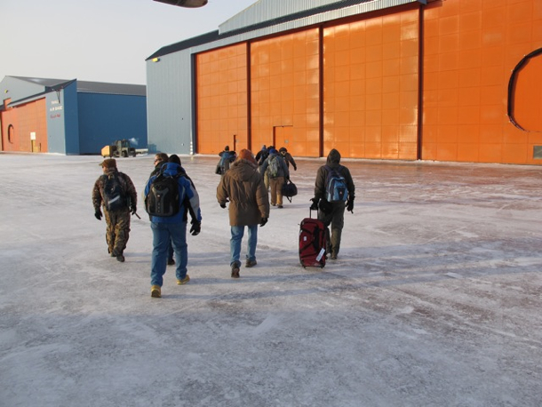
IceBridge teams arrive in cold and sunny Thule, Greenland. Credit: NASA/Jim Yungel
Back from Greenland, No Rest for the Weary
NASA and university partners returned from Greenland on May 28, concluding Operation IceBridge’s 2010 field campaign to survey Arctic ice sheets, glaciers and sea ice.
Over the span of almost 10 weeks, crew flew 28 science flights between the DC-8 and P-3 aircraft. Flight paths covered a total of 62,842 nautical miles, equivalent to about 2.5 trips around Earth at its equator. Credit: NASA
IceBridge — the largest airborne survey ever flown of Earth’s polar ice — has now completed two successive Arctic campaigns, adding a multitude of new information to the record from previous surveys.
Continue to follow the IceBridge blog and twitter feed to read updates as science results emerge. Also hear from scientists already planning the return to Antarctica this fall.
 IceBridge project scientist Michael Studinger, recently back from the field, offered words of thanks to those who helped made the 2010 Arctic campaign a success.
“A project of this size with two aircraft and multiple deployment sites and a fairly complex instrument payload is only possible with the support of many people. I would like to thank everyone from NASA’s Dryden Aircraft Operations Facility, NASA’s Wallops Flight Facility and NASA’s Earth Science Project Office, who all provided excellent support for Operation IceBridge. We also had excellent support from the NASA instrument teams, the science teams from the universities, and many of our science colleagues, both, from the teams in the field and from people back home in the labs. IceBridge also would like to thank the many people in Kangerlussuag and at Thule Air Base in Greenland who provided excellent support while we were there. We could not have accomplished our goals without their terrific help.”
Michael Studinger (right) readies for a science flight from Kangerlussuaq, Greenland, during the Arctic 2010 IceBridge field campaign. Credit: NASA/Jim Yungel
Seeing Eastern Greenland for the First Time
From: Jason Reimuller, aerospace engineering student, University of Colorado, Boulder
 My involvement with Operation IceBridge comes from a desire to better understand the polar climate and the climatic changes that are evident there. I have been working with NASA through the last five years as a system engineer for the Constellation project, while working to complete my doctoral dissertation in Aerospace Engineering Sciences at the University of Colorado in Boulder. I have also been recently involved with airborne remote sensing and LiDAR systems by completing a three year, NASA-funded research campaign that involved flying a small Mooney M20K aircraft to the Northwest Territories, Canada to better understand noctilucent clouds through synchronized observations with NASA’s Aeronomy of Ice in the Mesosphere (AIM) satellite.
This has been my first campaign with the project, participating in sorties based out of Kangerlussuaq, Greenland throughout the first two weeks of May 2010. To me, the project is a unique synthesis of personal interests — from polar climate observation and analysis, aircraft operations, remote sensing and instrument design, and flight research campaign planning. My role this year has been principally as a student with the intent to integrate the data that we collect with satellite and ground station data to better characterize glacial evolution, though I hope to become much more involved with the operations of future campaigns.
Seeing Eastern Greenland for the first time through the P-3’s windows, as its four engines lifting the aircraft easily over the sharp mountainous ridgelines and its strong airframe holding up to the constant moderate turbulence of the coastal winds being channeled through the fjords, was spectacular. I really got a strong sense of contrast between experiencing the stark minimalism of the ice cap and experiencing the aggressive terrain of the eastern fjordlands. The long flight trajectories we conducted there gave me a sense of the incredible diversity of the terrain and the low altitude of the flight plans gave me a connection to the environment not available at higher altitudes, even down to viewing the tracks of polar bears!
I have been very grateful to all the team members that have spent time with me to explain in detail the systems that they are responsible for, specifically the LiDAR systems, the photogrammetric systems, and the RADAR systems. Also, NASA pilot Shane Dover clearly explained to me the systems unique to the P-3 from a pilot perspective, which was of keen interest even though I may never log an hour in a P-3. In particular interest to me was the way John Sonntag was able to modulate complex flight plans onto ILS frequencies, providing the pilot a very logical, precise display to aid in navigating through both the numerous winding glaciers and the long swaths of satellite groundtrack. This has truly been an amazing personal experience, but upon hearing the excitement that many of the world’s top glaciologists have voiced about Operation IceBridge during my time in Kangerlussuaq, I’ve been proud to be a part of the team.
Ice Calves from Russell Glacier
From: Kathryn Hansen, NASA’s Earth Science News Team/Cryosphere Outreach Specialist

On May 14, 2010, scientists working from Kangerlussuaq, Greenland, with NASA’s IceBridge mission observed ice calving from nearby Russell Glacier. Credit: Eric Renaud/Sander Geophysics Ltd.
IceBridge scientists spend many days in flight surveying the snow and ice from above. On research “down days,” some scientists use their day off to take in the sights. On Friday, May 14, a group of scientists with Columbia University’s gravimeter instrument — which measures the shape of seawater-filled cavities at the edge of some major fast-moving major glacier — made the trek out to Russell Glacier. In the right place at the right time, the group witnessed a calving event that sent ice cascading down the glacier’s front.
“I took burst speed photos with my Canon 40D and just kept my finger on the trigger until everything stopped moving,” said Eric Renaud, an electronic technician with Sander Geophysics Ltd. “We were lucky to witness it.”
Read more about the group’s trek in a blog post by Columbia University’s Indrani Das, and watch a time-lapse video of the calving event composed by Renaud.
An Inland Connection?
From: Kathryn Hansen, NASA’s Earth Science News Team/Cryosphere Outreach Specialist
 Scientists have long been tracking Greenland’s outlet glaciers, yet aspects of glacier dynamics remain a mystery. One school of thought was that glaciers react to local forces, such as the shape of the terrain below. Then, researchers noticed that glaciers in different regions were all thinning together, implying a connection beyond local influences. Scientists have posed theories about what that connection might be, but the jury is still out.
Recently, the landscape in southeast Greenland has started to change. Helheim Glacer, which was thinning at 20-40 meters per year, slowed dramatically to just 3 meters per year while thinning of the nearby Kangerdlugsuaq also slowed. Further south, two neighboring glaciers showed the opposite trend and started thickening by as much as 14 meters per year. Neighboring glaciers behaving in similar ways implies a connection, but what exactly?
The IceBridge flight on May 12 will help scientists learn how changes to outlet glaciers affect the ice sheet inland. Instruments on the P-3 surveyed in detail three southeast glaciers: Fridtjof-Nansen, Mogens North and Mogens South. Next they flew four long lines mapping changes near the ocean and up to 60 kilometers inland, capturing the extent, if any, at which thinning near coast reflects on changes to the ice inland. It’s an important connection to make; while the loss of outlet glaciers alone would not contribute much to sea level rise, loss of the ice sheet could have a dramatic impact.
IceBridge crew and researchers board the P-3 on May 12 for a flight to study glaciers and the ice sheet in southeast Greenland. Credit: NASA/Kathryn Hansen
 |
 |
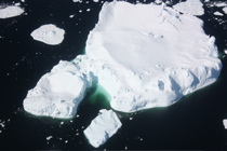 |
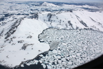
The P-3 flew over areas of sea ice wile mapping glaciers and the flight line closets to the coast. Credit: NASA/Kathryn Hansen
 |
 |
 |
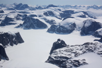
Mountainous terrain along Greenland’s southeast coast led to short-lived periods of turbulence and spectacular scenery. Credit: NASA/Kathryn Hansen