science – Page 3 – Operation IceBridge

Airborne education: Science teachers in Kangerlussuaq

By George Hale, IceBridge Science Outreach Coordinator, NASA Goddard Space Flight Center

This year’s Arctic campaign distinguishes itself from previous ones by welcoming visiting teachers from the United States, Denmark and Greenland. Through cooperation with the U.S. Embassy in Copenhagen, the Danish Ministry of Education and the National Science Foundation’s PolarTREC program, five teachers—two from Denmark, two from Greenland and one from the United States—were chosen to join Operation IceBridge in April.

These teachers will be embedded with the IceBridge team for several days, staying with IceBridge personnel in the KISS facility, riding along on survey flights and attending daily science meetings. The teachers will trade off days flying and days on the ground during their stay, with activities such as a glacier field trip and excursion to a nearby fossil site.

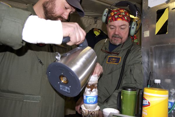
From left: Teachers Peter Gross, Erik Jakobsen and Tim Spuck, and CReSIS instrument team member Aqsa Patel examine the day’s planned survey route. Credit: NASA/Jefferson Beck

Meet the teachers

Peter Gross is a physics and math teacher at the Roskilde Technical Gymnasium in Roskilde, Denmark. Gross uses the science and math skills he gained in his education and during his time as an engineer and his tremendous enthusiasm for teaching to educate a new generation of science, technology and mathematics (STEM) students.

Erik Winther Jakobsen teaches at the Aalborg Gymnasium in Aalborg, Denmark, and has for the past several years worked on the subject of human environmental impacts and climate change. While working on and teaching this subject, Jakobsen noticed a need for more reliable time-series data on ice sheets, something Operation IceBridge is working to achieve.

Sine Madsen has been teaching biology with an emphasis on climate change in the Arctic at the Building and Construction school in Sisimiut, Greenland, for the past 10 years. Madsen hopes to use her new knowledge about how climate is changing in the Arctic and share these insights with her students back home.

Tom Koch Svennesen is a chemistry and comparative religion teacher at Aasiaat GU in Aasiaat, Greenland. Svennesen has seen firsthand how the ice in Greenland has changed in recent years. In his time teaching in Greenland, he has faced a variety of challenges such as the disadvantages faced by Greenlandic youth whose parents don’t speak Danish and thus have a harder time learning the language used in Greenland’s education system.

Tim Spuck joins IceBridge as part of NSF’s PolarTREC program, an effort designed to embed science teachers in with scientists doing polar research. Spuck teaches science in Oil City, Penn., and aims to use what he’s learned through the program to better reach STEM students in his school.

The Greenlandic and Danish educators arrived in Kangerlussuaq on April 13 and leave on April 19. Spuck got there the following day and will remain with IceBridge until April 25. After landing, teachers had a chance to see the town, buy groceries and settle into their rooms in the KISS facility before heading to the airport to greet the returning P-3. After the April 13 flight, the teachers sat in on IceBridge’s daily science meeting, where they introduced themselves to the team and decided who among them would be the first to join a survey flight.

Teachers getting an explanation of DMS

DMS team member James Jacobson (left) explains the basics of the P-3’s Digital Mapping System to Tom Koch Svennesen and Peter Gross. Credit: NASA/Jefferson Beck.

In the air and on the ground

On the morning of April 14, Svennesen and Gross boarded the plane, and after a quick safety briefing by the flight crew, strapped into their seats for the Helheim-Kangerdlugssuaq Gap survey. On this flight, the P-3 would quickly transit the ice sheet and start a series of roughly north-south runs across several glaciers on the east coast of Greenland. This survey, informally known as mowing the lawn, would start close to the shore, gradually moving inland with each pass.

This flight yielded a large amount of data for IceBridge scientists and many sightseeing and photo opportunities for everyone on the plane. Unfortunately, the flight had to be cut short a little early due to concerns about a possible fuel leak in one of the engines. The P-3’s flight crew noticed streaks coming from the engine that could have indicated a leak and the pilots returned directly to Kangerlussuaq as a precaution. After an extensive engine test, the flight crew determined that what they saw was water from melting ice that caused the steaks.

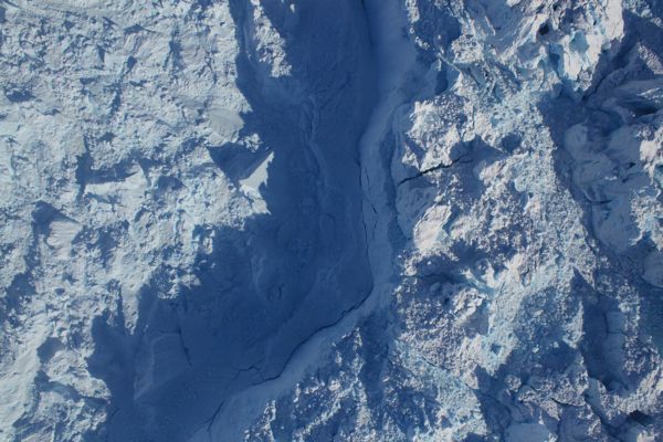
On Sunday the airport was closed, meaning a well-deserved day off for the P-3 flight crew. Without a flight, many IceBridge people, including the teachers, took advantage of their time on the ground to visit the nearby Russell Glacier. The trip gave teachers and scientists a chance to interact, take lots of photos and see part of the Greenland ice sheet up close. That evening, after a busy and windy day of hiking around the ice, everyone gathered for a group dinner in the downstairs kitchen of the KISS facility, which gave teachers more opportunity to learn from scientists and each other.

Early on April 16, Madsen, Spuck and Jakobsen—who didn’t get to fly on Saturday—joined the IceBridge team on another flight, this one a grid survey of glaciers in the Geikie peninsula. At the last minute, an extra seat opened on the P-3, and Gross joined the group while Svennesen stayed behind to work on the website he runs for his students. Despite a fair amount of cloud cover for part of the flight, this survey was another in a long line of IceBridge successes, with ATM only losing about five percent of its data due to clouds. When asked about his favorite moment during the flight, Jakobsen said he enjoyed seeing the interesting geology of the Geikie peninsula and, of course, the pitching maneuvers used to calibrate the radar.

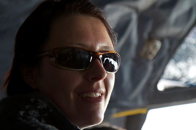
Sine Madsen sits in a jump seat in the P-3 cockpit during an IceBridge survey flight. Credit: NASA/Jefferson Beck

Teachable moments

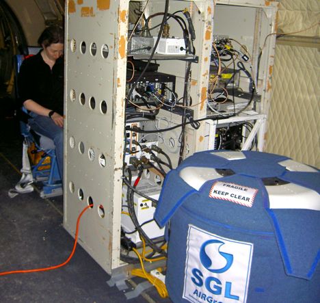
On each flight the teachers take advantage of opportunities to talk to the science and instrument teams on board. Shortly after takeoff on both flights, ATM program manager Jim Yungel gave a detailed explanation of the inner workings of the Airborne Topographic Mapper and the science behind using lasers to determine ice surface elevation from the air. They also got to learn more about the Digital Mapping System, gravimeter and magnetometer, and the P-3’s various radar instruments.

The IceBridge experience continued even on non-flight days. During and after a group dinner on Sunday, teachers talked with several members of the science and instrument teams, learning more about IceBridge’s instruments and polar science. Having educators working with scientists and living in the same facility allows for many of these informal question-and-answer sessions, which are often more enlightening than a lecture or information session, and gives them a taste of life as a polar scientist. The experience has also given these teachers new ideas for ways to teach science to their students in ways that are based on real world examples.

Witnessing the last P-3 Arctic sea ice flight for 2012

By George Hale, IceBridge Science Outreach Coordinator, NASA Goddard Space Flight Center

The transfer of IceBridge’s base of operations from Thule to Kangerlussuaq normally marks the end of sea ice surveys done by the P-3 for the campaign. At this time, scientists on the P-3 change their focus toward ice sheets and glaciers, while researchers aboard the Falcon jet using Land, Vegetation and Ice Sensor (LVIS) will continue studying sea ice. But with starting the campaign with a transit to Alaska and beginning operations in Kangerlussuaq by crunching data on the ground while the P-3 is in Wallops being repaired, this year has been anything but ordinary. I’ve been asked to give my views as a newcomer to IceBridge and first-time visitor to the Arctic and I’m happy to share.

First, I have to state that while I have a basic background and interest in science, I’m not a scientist by training. My role as a communicator is not to make scientific discoveries, but to spread the word about them. Part of my job as IceBridge’s science outreach coordinator is to help bridge the gap between what scientists find and what the public understands.

Being outside of the science of sea ice gives me a different perspective on things. I’ve been keeping up with news from the Arctic campaign, but it wasn’t until actually riding along on a sea ice flight that I felt I knew what was happening. Being with scientists as they gather data and sharing the flight experience with them will hopefully help me improve IceBridge’s educational and public outreach efforts.

New to the Program

I arrived in Kangerlussuaq on April 9, the same day as the P-3 returned from Wallops. While flying from Thule the week before, the P-3 started having issues with one of its engines, something unavoidable with the workload and conditions the P-3 is subjected to. In the interest of safety, the pilots shut the engine down and flew directly into Kangerlussuaq. After a one-day delay because of weather, the P-3 made its way back to the Wallops Flight Facility in Virginia for an engine replacement.

The P-3’s return flight to Greenland coincided with my scheduled arrival there, so I was extended an invitation to ride along. Unfortunately, this didn’t work with the arrangements for my commercial return flight, so I wasn’t able to go. I arrived in Kangerlussuaq on an Air Greenland flight Monday morning with enough time to unpack, check my email and buy some groceries before joining others at the airport to see the P-3 arrive.

Bright and early Tuesday morning, I joined 23 other people in braving the 12 degree Fahrenheit weather to board the P-3 for one last sea ice flight along the east coast of Greenland that would put us on an intersecting path with the NASA ER-2 carrying MABEL. At this point in the campaign, IceBridge normally flies glacier surveys, but weather conditions made that unfeasible.

A map of the 2012 Arctic campaign’s sea ice flight. Credit: Michael Studinger/NASA

Sea Ice in Review

This flight was another in a long line of successful sea ice surveys and joint operations with other aircraft. IceBridge has flown 15 sea ice flights, including several along CryoSat orbits and two joint flights with aircraft from the European Space Agency as part of CryoVEx, their CryoSat validation campaign.

Aside from the highly successful joint ESA/NASA flights, this year’s Arctic campaign stands out as completing several more sea ice flights than previous years, covering a distance greater than the circumference of the Earth around the equator. In total, IceBridge has collected huge amounts of sea ice data from instruments like ATM, DMS and the new KT-19 temperature sensor used for sea ice lead detection.

And this data is just sitting around waiting to be processed. This year IceBridge scientists are working to build a quick sea ice product from information that’s only days old. If this proves successful, it has the potential to improve sea ice forecasts and statements for the general public. IceBridge scientist Nathan Kurtz talks about his work with sea ice and the quick sea ice product in his earlier blog post.

A diagram showing sea ice thickness and the role snow cover plays

Having successes like these early on sets the bar for the rest of the campaign, and after hearing about IceBridge’s success for several weeks, I now get the chance to witness it first-hand.

My First Sea Ice Flight

I’ve been hearing about IceBridge’s campaign successes since operations began in March. Knowing I would join the team in April and get to see these successes first-hand was very exciting. Being there as things happen promises to be a great experience, and I can only hope to avoid getting in the way. On the morning of my first survey flight, I strap into my seat. I’m not entirely sure what to expect, but I’m ready to see IceBridge at work.

I am in some ways grateful that my first flight was over sea ice. Although it may have been a letdown for those who have flown many sea ice flights this year already, I was glad to have a relatively gentle introduction. Compared to glacier surveys, sea ice flights are smooth and easy, with no crosswinds coming out of fjords and far less turbulence.

As I walked around the cabin I saw members of the IceBridge team working diligently, recording data and making necessary adjustments to their instruments. I also looked out the P-3’s side windows to watch sea ice as we passed 1,500 feet overhead. The flight wasn’t all straight and level though. The pilots put the P-3 through a series of pitching and rolling maneuvers at higher altitude for instrument calibration. The up and down parabolic arcs and resulting feeling of lessened gravity seem to be a favorite, bringing smiles to the faces of both novices such as myself and IceBridge veterans.

A Cold Ride Home

Several hours later we returned to the airport, with the bulk of the team ready to get off the plane and warm up. During the return leg a mechanical issue caused the plane’s climate control to start blowing cold air instead of warm. By the end of the flight, it was around 40 degrees Fahrenheit in the back of the cabin and some bottles of water sitting on the deck were starting to form ice on the bottom.

After landing we take a short break (to warm up) and then head off to the daily science meeting, where we discuss the day’s events and look at weather forecasts to make plans for tomorrow’s flight. The plan is to survey some of the eastern glaciers, which means a more turbulent flight for my second day on the P-3. I’m looking forward to riding along on as many flights as I can in the following days, and to working with the American, Danish and Greenlandic teachers arriving soon to participate in IceBridge.

Synchronized NASA and ESA flights across Arctic Ocean — a success!

By Malcolm Davidson/ESA and Michael Studinger/NASA

Arctic sea-ice from the NASA P-3 (NASA/M. Studinger)

Monday April 2 has been much anticipated bythe teams in Thule, Greenland (NASA) and Alert, Canada (ESA). While the objectivesfor the day were clear – jointly fly with all available planes beneath CryoSat’searly morning pass over the Arctic Ocean – the execution of such flights is andalways will be a challenge.

Flying joint multi-plane missions is arather daunting task. Departure and rendezvous times and locations need to becalculated and maintained to ensure that the instruments on the differentplanes will see the same sea-ice floes below (these move after all), flightaltitudes need to be established and maintained for safety reasons, instrumentsneed to be warmed up and ready ‘in-time’, somewhat grumpy firefighters need tobe coaxed out to the airstrip ahead of working hours to support an earlydeparture and the list goes on.

With both teams committed to the flights,the first task early this morning was to check the weather forecast for theday. These proved to be good with temperatures of –29°C (–20°F) and generally clear skies; but not ideal! Some rather worryingcloud formations featured near the coast in satellite images.

NASA P-3 cockpit

NASA P-3 cockpit (NASA/M. Studinger)

Nevertheless, after a quick phone callbetween the NASA and ESA coordinators (at a time before most people have yet toreach for their mug of morning coffee) the decision was made: it’s a go.

From then on it there was a flurry ofactivity on both sides, pilots warmed up their planes, instrument teams checkedout their instruments, flight plans were programmed into the onboard computersand so on.

Twin Otter takes off

The NASA P-3 plane was the first to go out, leaving Thule a full hour before the two ESA planes located closer to the track. On the tarmac in Alert there was the first casualty of the day – despite heroic efforts the EM-bird ice-thickness instrument could not be coaxed into life. The die was cast – the second Twin-Otter plane would have to go it alone and meet up with the NASA P-3.

NASA’s sea-ice mission plan for April 2 (yellow). We teamed up with ESA at 10520 north of Alert. (NASA/M. Studinger)

Around 07:30 (local time) the CryoSat satellite – always on schedule – ripped above the Arctic Ocean taking about one minute to race along the 500-km (310 mile) transect that would later take several hours of plane time to cover.

At 08:00 both the ESA and NASA planes reached the edge of the Arctic Ocean almost simultaneously and headed across the sea ice flying exactly along the same line that CryoSat had just covered. The timing was so good that, for the first time, there was visual contact between the planes, a remarkable achievement!

The image below, which is a DMS mosaic from Eric Fraim shows one of the many leads we saw from the NASA P-3 today with a variety of different types of sea ice.

DMS mosaic of lead in the sea ice

DMS mosaic of lead in the sea ice (NASA/DMS/E. Fraim)

The rest of the day turned out very well indeed. The clouds that had worried the teams in the morning only formed only a thin band near the coast. The rest of the line out on the ocean was clear and beautifully lit by the oblique Arctic Sun. All the onboard scientific instruments on both planes worked well so that by the end of the day it was clear that the day had been a success.

By joining forces both the ESA and NASA teams collected a highly valuable dataset that will benefit the scientific achievements of ESA’s CryoSat and NASA’s future ICESat-2 mission to better monitor sea ice from space.

For more about ESA’s CryoSat mission and CryoVEx campaign, visit their Campaign Earth blog

In the spirit of international collaboration: Honoring the Terra Nova Expedition

By Michael Studinger, IceBridge Project Scientist, NASA Goddard Space Flight Center/UMBC

Thule Air Base, Greenland – March 29, 2012 is a special day for polar researchers worldwide. It marks the centennial of Sir Robert Falcon Scott’s death on the Ross Ice Shelf. Many commemorative events have taken place around the world to remember the scientific accomplishments of the Terra Nova Expedition, particularly those of the Pole Party consisting of Robert Falcon Scott, Edward Wilson, Henry Bowers, Lawrence Oates and Edgar Evans. The most prominent event was a National Service of Commemoration for Captain Scott and the Pole Party at St. Paul’s Cathedral in London, with IceBridge’s own Seelye Martin attending as a guest of honor.

In 2008 I had the privilege to visit Captain Scott’s historic Terra Nova Hut on Cape Evans in Antarctica, and the geographic South Pole, where the National Science Foundation installed a sign bearing Scott’s famous quote said when the party realized the Norwegian expedition, led by Roald Amundsen, had been there first: “The pole. Yes, but under very different circumstances from those expected.” These are moments in my life that I will never forget. Walking through the Terra Nova Hut, which looked like it has been frozen in time, took my breath away.

Inside Captain Scott’s Terra Nova Hut on Cape Evans. The hut was built in 1911 by members of the British Antarctic Expedition (Terra Nova Expedition) and used as base for the trek to South Pole from which Scott and four of his team members never returned. The hut is remarkably well preserved but is undergoing restoration by the Antarctic Heritage Trust to protect it from further decay. The kitchen area on the left is one of the many areas inside and outside the hut that are being worked on. The hut is part of the 100 most endangered sites on the World Monuments Watch List. It is a remarkable place to be to say the least. Credit: Michael Studinger/NASA.

One hundred years later polar research has changed dramatically. On the day of the centennial, NASA’s Operation IceBridge and the European Space Agency’s CryoVEx campaign coordinated flights of two aircraft from different locations over the Arctic Ocean on a track flown shortly before by ESA’s CryoSat-2 spacecraft 600 km (370 miles) above us. We are able to do this because we have modern satellite images that are a few hours old and computer models showing the cloud cover in the survey area. We have modern means of communication that allow us to coordinate these science flights a few hours before takeoff. We know our position within a few feet and the NASA Airborne Science program flight tracker shows our position in real time. A lot has changed to say the least, but nevertheless operating in the remote polar regions remains a challenge even today. Modern navigation computers routinely get confused within a few miles of either the North or South Pole, the extreme cold still poses a challenge and weather predictions can be wrong. The safety and success of our operations is only possible because of extremely experienced and skilled members of the aircrew and instrument teams that excel in meeting the challenges of the polar environment every day.

McMurdo Station in Antarctica with the historic Discovery Hut in the foreground. The hut was built during Scott’s 1901-1903 expedition. The contrast between old and new is amazing. Observation Hill, the site of the Terra Nova memorial cross can be seen in the background on the right. Credit: Michael Studinger/NASA.

Today’s polar research is driven by a spirit of international collaboration and the joint NASA/ESA flight on March 29, 2012 is a fine example of what can be accomplished when many nations and organizations team up instead of competing with each other. Recognizing the enormous accomplishments of the early polar explorers, we dedicate this flight to the members of the Terra Nova Expedition, who died in Antarctica one hundred years ago.

NASA P-3 flight path

Flight path of the NASA P-3 Orion in yellow during the joint sea ice science mission with ESA’s CryoVEx airborne campaign stationed in Alert on Ellesmere Island and CryoSat-2.

New perspectives on the IceBridge sea ice campaign

By Nathan Kurtz, IceBridge scientist, NASA Goddard Space Flight Center/Morgan State Univ.

As the IceBridge Arctic sea ice campaign continues another successful year, I’ve been given this wonderful opportunity to discuss my experiences on the mission, and more importantly, how they relate to the critical science questions that need to be answered. I realize that there are many details I find intriguing as a scientist that are inherently uninteresting to non-scientists, so I won’t wax philosophical about how impressed I was to see things like the self-similar structure of deformation patterns in sea ice (if you actually came here for that, I apologize). My aim is to communicate the importance of what we are learning to the broader public who funds and ultimately benefits from this work. I hope you learn something about why we are devoting so many resources to this scientific study, as this is perhaps the most effective type of ‘bridge’ the IceBridge mission can make: to raise awareness of the state of the climate and present the scientific facts as we have gathered them through a long and arduous field campaign.

IceBridge science team member Nathan Kurtz checking out the sea ice conditions

IceBridge science team member Nathan Kurtz checking out the sea ice conditions. Credit: James Yungel/NASA.

This was my first trip to the ice-covered regions of the Arctic and I fully admit to reverting back to an excited childlike state of wonder as my initial flight to Thule, Greenland, touched down. It was quite striking to take in the sight of the vast snow-covered mountains and frozen sea, feel the bitter cold draining the heat and life from my body and realize that actual ‘monsters’ with an instinctive mindset to view humans as prey were all around. But I was shocked to see a hardened community of people standing resolute against these elements. Even more shocking, was to imagine why humans came here thousands of years ago without modern technology. What led them here? For me, the Arctic has always symbolized the unknown, but with hidden treasures awaiting anyone brave enough to explore it. But I realize my subjective symbolic interpretation is also remarkably universal in that native settlers, polar explorers and scientists must also have come to the Arctic with a desire to explore an unknown wilderness and gain some new knowledge from their experience.

On the scientific end of this knowledge spectrum, recent studies have increasingly shown the importance of the Arctic to the climate. The once seemingly insignificant and remote Arctic region is now understood to be intimately connected to the rest of the planet. Sea ice variability affecting the severity of snow storms in Europe, melting sea ice increasing the absorption of sunlight by the Earth and melting ice sheets causing sea level rise are but a few of many such connections. We are learning that what happens in the Arctic will profoundly affect the whole of humanity all over the Earth. Viewed in this way, it is no longer a coincidence that humans have taken such a keen interest in the Arctic, and that this wild frontier is indeed a source of valuable knowledge waiting to be unearthed.

Looking out across the sea ice near Thule, Greenland

Looking out across the sea ice near Thule, Greenland. Credit: Nathan Kurtz/NASA

As a scientist, the purpose of my trip here is to learn more about the Arctic sea ice cover. My job is to use a combination of lasers, radars, cameras and infrared sensors to determine how the thickness of sea ice is changing, and whether any observed changes can be linked to the larger climate system. Flying over the sea ice with all the IceBridge instruments operating simultaneously has given me a whole new perspective on the mission. It has taken me from my normal desk job of looking at numbers on a computer screen, to the reality of what those numbers represent, and back again full-circle to connecting these concepts in a meaningful way. It has given me the opportunity to physically see that an increased laser surface elevation is actually a large sea ice pressure ridge, a widely spaced radar return is actually a snow drift. That, ultimately, all of the IceBridge results are indeed real and meaningful. It is this connection between numbers on a computer screen to the reality of the ground which will provide me and other scientists with the ability to come up with a rigorous scientific explanation of precisely what role sea ice thickness changes will have on the climate.

In the course of my own analysis of the IceBridge data I have been constantly questioning my methods to ensure that my excursions into the abstract realm of mathematical and scientific theory do not lose sight of this connection to the things I’ve seen on the ground. Questions such as what do I do when I try to invert a matrix of IceBridge data and it explodes? How can I utilize statistics to determine just how accurate these measurements are? Are my solutions to these problems in tune with the physical environment I have witnessed? This ultimately translates into maintaining high standards and objectivity, which is critical to any scientific research area.

Sunrise over sea ice near the North Pole

Sunrise over sea ice near the North Pole. Credit: James Yungel/NASA

But this is, admittedly, my own subjective understanding of my role in this project. More important, is how my understanding and use of these concepts relates to the scientific results being obtained, and how these results can then be translated into a general statement for the public such as ‘the sea ice thickness decreased by x centimeters’ Towards this end, I and a large team of people have worked for the past two years on developing methods to turn the instrument data from IceBridge into clear and understandable scientific data products. We recently reached a major milestone in the project by demonstrating our ability to produce easy to understand products such as snow depth and sea ice thickness from past missions. In the interest of promoting honest and open exchange of scientific knowledge, we have given public access to these data sets (http://nsidc.org/data/idcsi2.html) in such a way that anyone can look at the latest results of the project. In doing so, we went from the realm of raw instrument data, to something that anyone can understand and interpret.

To further improve the utility of the IceBridge sea ice campaigns, we are attempting an unprecedented feat: to produce a quick version of the scientific products to support operational forecasting of sea ice. This is shaping up to be a monumental undertaking, and we are working hard to understand how to work with days-old field data. It remains to be seen what role IceBridge can play in sea ice forecasting and how we can interpret the data to come up with statements about the state of Arctic sea ice for the general public. But, so far the results from the first few flights look fantastic! We have also provided our preliminary results to support an ESA sponsored campaign conducting field missions in the area. Everything is proceeding in a positive direction, so stay tuned for more updates as the IceBridge mission continues!

Operation IceBridge surveys new areas in the Beaufort and Chukchi Seas north of Alaska

By Michael Studinger, IceBridge Project Scientist, NASA Goddard Space Flight Center/UMBC

Fairbanks, AK – The two most important sea ice flights every year are two crossings of the entire Arctic Basin, north of Greenland and Canada all the way to Alaska. This year we decided to make the flights to and from Fairbanks earlier than usual because of the weather. The forecast at Thule was predicting a major storm system for the next few days. Storm season in Thule lasts Sept. 15–May 15, and every year blizzards with wind speeds of over 100 miles per hour and white out conditions hit the base, locking us down for a few days.

There are several challenges involved with these two flights. First, the survey lines are 1600 miles long and it is very rare to have such a large area free of clouds and fog, particularly over the Arctic Ocean. Imagine flying from New York to Colorado at 1500 feet above the surface and having neither clouds nor fog the whole way. Getting good data from our optical sensors, such as laser altimeters and digital cameras, we need clear conditions between the aircraft and the ice surface.

IceBridgeflight from Thule, Greenland to Fairbanks, AK that surveyed sea ice along atransect over the entire Arctic Basin. Basemap is MODIS satellite image showingcloud cover and sea ice over the Arctic Ocean.

A second challenge comes from predicting the weather in such a remote area. We have infrared satellite images and computer models available, but these models cannot be validated because there are no weather stations in the Arctic Ocean. Also, neither the forecast models nor satellite images show the weather features that are most important to us: low clouds and ice fog that disrupt the laser and camera measurements.

The third challenge is that we have to relocate the aircraft, crew and scientists to Fairbanks on very short notice, since the frequent changes in weather allow us to make this decision only a few hours before takeoff.

The NASA P-3 aircraft is being prepared on a chilly morning for a sea ice mission over the Beaufort and Chukchi Seas from Fairbanks, Alaska. Photo: Michael Studinger/NASA.

TheNASA P-3 aircraft is being prepared on a chilly morning for a sea ice missionover the Beaufort and Chukchi Seas from Fairbanks, Alaska. Photo: MichaelStudinger/NASA.

In order to characterize the state of the Arctic ice pack we need to survey large regions and determine the thickness of the multiyear ice that remains from the previous summer and the growth of new first year ice during the winter. We have had several successful flights over the Beaufort and Chukchi Seas from Fairbanks that surveyed primarily the newly formed first year ice in this area. This is a new area for IceBridge and an important data set to monitor changes in the Arctic environment.

We are planning to stay here in Fairbanks for a few more days before we return to Thule Air Base in Greenland to continue our campaign and survey the sea ice north of Greenland.

The margin of a large lead of open water (dark) and thingrease ice (gray, right) in the Chukchi Sea between Alaska and Russia. Theimage was create using several frames from the Digital Mapping System (DMS)onboard the NASA P-3. Image: NASA/DMS/Eric Fraim.

Ice Cap Recap

From: Kathryn Hansen, NASA’s Earth Science News Team / Cryosphere Outreach

May 16, 2011

Last month, IceBridge surveyed Sukkertoppen Ice Cap — a mass of ice southwest of the mission’s base in Kangerlussuaq, Greenland. I didn’t know what to expect from an ice cap. Would it resemble the vast, white expanse of the Greenland Ice Sheet next door?

At the surface, Sukkertoppen looked remarkably like an ice sheet. After all, both form from the accumulation of snow compacted over thousands of years. Before long we reached the rugged mountains and blue-green fjord that separates the cap from the main ice sheet, and we turned back for another pass.

On April 8, 2011, IceBridge flew a mission to coastal areas in southwest Greenland. Mountains and an open-water fjord surround one of the mission’s targets, a small ice cap called Sukkertoppen Isflade. Credit: NASA/Michael Studinger

Ice caps are simply small versions of ice sheets, measuring in at a maximum area of 50,000 square kilometers (about 19,000 square miles). Anything larger is considered an ice sheet. They’re also thinner. It’s their small stature that makes ice caps more prone to melt in a warming Arctic.

Charles Webb of NASA’s Goddard Space Flight Center in Greenbelt, Md., explains the importance of monitoring ice caps in the Canadian Arctic. Credit: NASA/Jefferson Beck

South of Sukkertoppen lies the Canadian Arctic – home to the largest amount of ice outside of Greenland and Antarctica and contributing significantly to sea level rise.

IceBridge is adding to the long-term record of changes to the ice caps. On May 5, IceBridge surveyed the Devon Ice Cap – among the Canadian Arctic’s top ten largest caps. Then on May 10, the P-3 surveyed several glaciers and small ice caps on Ellesmere Island, Axel Heiberg Island and Meighen Island, including the Prince of Whales Ice Field and the Agassiz Ice Cap.

Finally on May 12, IceBridge surveyed the Barnes Ice Cap. Barnes is a curiosity because it is considered a significant remnant of the vast Laurentide Ice Sheet the covered most of Northeast America and Canada during the last glacial. NASA previously used the ATM laser altimeter to map the ice cap in 1995, 2000 and 2005, showing a slight acceleration in thinning of the ice cap.

“It’s our hope that by combining these data sets we’ll have a long term time series about whats happening there so we can better understand the dynamic of the ice caps as well as use them as early warning indicators of what is happening in our climate,” said Charles Webb of NASA’s Goddard Space Flight Center in Greenbelt, Md.

On May 12, IceBridge surveyed Barnes Ice Cap on Baffin Island. In addition to mapping its surface elevation, instruments also measured the bedrock topography, which will allow scientists to better model ice dynamics and estimate when the Barnes Ice Cap will be completely melted. Credit: NASA/Michael Studinger

Measuring Gravity From a Moving Aircraft

From: Joël Dubé, Engineer/Geophysicist at Sander Geophysics, OIB P-3 Gravity Team

One of the instruments used in Operation IceBridge (OIB) is an airborne gravimeter operated through a collaboration between Lamont Doherty Earth Observatory of Columbia University and Sander Geophysics. Some people from other instrument teams call it a gravity meter, gravity, gravitometer, gravy meter, gravel meter, gravitron, or blue couch-like instrument. As operators of the gravimeter, we are referred to as graviteers, gravi-geeks or gravi-gods. This tells a lot about how mysterious and unknown this technology appears.

Let me summarize the basics of airborne gravity data acquisition for you.

But first, why is gravity data being acquired as part of OIB?

The earth’s gravity field is varying in space according to variations in topography and density distribution under the earth’s surface. Essentially, the greatest density contrast is between air (0.001 g/cc), water and ice (1.00 and 0.92 g/cc, respectively) and rocks (2.67 g/cc in average). Therefore, gravity data can be used for modelling the interface between these three elements. The ATM system (laser scanner) can locate the interface between air and whatever is underneath it with great accuracy. The MCoRDS system (ice penetrating radar) is successful at locating the interface underneath the ice. However, no radar system can “see” through water from the air. Hence, gravity data can help determine bathymetry beneath floating ice, either off shore or on shore (sub-glacial lakes). This in turn enables the creation of water circulation models and helps to predict melting of the ice from underneath. Also, airborne gravity data can contribute to increasing the accuracy and resolution of the Earth Gravitational Model (EGM), which is determined only with low resolution in remote locations such as the poles, being built mainly from data acquired with satellites.

Most people don’t know that it is possible to acquire accurate gravity data from a moving platform such as an aircraft. Due to the vibrations and accelerations experienced by the aircraft, it is definitively a challenge! There are four key elements that make this possible.

1- You must have very accurate acceleration sensors, called accelerometers.

2- You must keep these accelerometers as stable as possible, and oriented in a fixed direction. This is a job for gyroscopes coupled with a system of motors that keeps the accelerometers fixed in an inertial reference frame, independently of the attitude of the aircraft. This is why the system we use is called AIRGrav, which stands for Airborne Inertially Referenced Gravimeter. Damping is also necessary to reduce transmission of aircraft vibrations to the sensors. The internal temperature of the gravimeter also has to be kept very stable.

This is all good. However, the accelerations we are measuring this way are not only due to the earth’s gravity pull, but also (and mostly) due to the aircraft motion. And to correct for that:

3- You need very accurate GPS data, so that you can model the aircraft motion with great precision.

Despite these best efforts, noise remains, mostly from GPS inaccuracies and aircraft vibrations that can’t be detected by GPS, so:

4- You have to apply a low pass filter to the data, since the noise amplitude is greatest at high frequency.

The AIRGrav system on-board the P-3 aircraft. Gravimeter (right), rack equipped with computers controlling the gravimeter and GPS receivers (center) and operator (left). Credit: Joël Dubé

Furthermore, a number of corrections have to be applied to the data before they can serve the scientific community. The corrections aim at removing vertical accelerations that have nothing to do with the density distribution at the earth’s sub-surface.

The Latitude correction removes the gravity component that is only dependent on latitude. That is the gravity value that would be observed if the earth was treated as a perfect, homogeneous, rotating ellipsoid. This value is also called the normal gravity. Since the earth is flatter at the poles, being at high latitude means you are closer to the earth’s mass center, hence the stronger gravity. Also, because of the earth’s rotation and the shorter distance to the spinning axis, a point close to the pole moves slower and this will add to gravity as well (less centrifugal force acting against earth’s pull).

Anything traveling in the same direction as the earth’s rotation (eastward), will experience a stronger centrifugal force thus a weaker gravity, and the other way around in the other direction. Traveling over a curved surface also reduces gravity no matter which direction is flown, similar to feeling lighter on a roller coaster as you come over the top of a hill. This is known as the Eötvös effect and is taken care of by the Eötvös correction. This correction is particularly important for measurements taken from an aircraft moving at 250-300 knots.

The Free Air correction simply accounts for the elevation at which a measurement is taken. The further you are from the earth’s center, the weaker the gravity.

To give you an idea of how small the gravity signal that we are interested in is with respect to other vertical accelerations that have to be removed, let’s look at the following profiles made from a real data set. All numbers are in mGals (1 m/s2 = 100,000 mGals), except for the terrain and flying height which are in meters.

A visual summary of gravity corrections. Credit: Stefan Elieff

“Raw Gravity” in this diagram means that GPS accelerations (aircraft motions) have been removed from inertial accelerations. Notice the relative scales of the profiles, starting at 200,000 mGals, down to 20,000 mGals when aircraft motions are accounted for, down to 200 mGals after removing most of the high frequency noise, and ending at 50 mGals for Free Air corrected gravity. Free Air gravity is influenced by the air/water/ice/rock interfaces described earlier, and since OIB uses the gravity data to find the rock interface (the unknown), Free Air gravity is the final product. As a side note, for other types of gravity surveys, we usually want to correct for the terrain effect (the air/water/rock interfaces are known in these cases), so that we are left with the gravity influenced only by the variations of density within the rocks. This is called Bouguer gravity and is also shown in the figure.

Notice the inverse correspondence between flying height (last profile, in blue) and the profiles before the free air correction (going higher, further from the earth, decreases gravity), and the correspondence between terrain (last profile, in black) and the free air corrected data.

Now, let’s look at some data acquired during the current 2011 mission in western Greenland.

Ice elevation (left), rock elevation (middle) and Free Air gravity data (right). Greenland 2011 flight lines shown in black. Gravity data is preliminary and is not yet available for scientific analysis.

The left panel shows the elevation of the rocks, or of the ice where ice is present. It is as if the water has been drained from the ocean. The middle panel shows only the bedrock elevation, both ice and water being removed. The data is from ETOPO1, a global relief model covering the entire earth. The right panel shows the Free Air gravity acquired in the last few weeks. Most channels, called fjords, are well mapped by the gravity data. It is interesting to see that the gravity data infers the presence of a sub-glacial channel (shown by the red arrow) where no channel is mapped (yet?) on the bedrock map. The most likely reason for this is that this particular region has not been covered by previous ice radar surveys (there are huge portions of the Greenland ice sheet that remain unexplored). Note that the MCoRDS ice radar data acquired as part of the current campaign will improve the resolution in this area and will enable for a better comparison of both data sets in the future.

Battling the Arctic Chill

From: Kathryn Hansen, NASA’s Earth Science News Team/Cryosphere Outreach

April 6, 2011

Kangerlussuaq, Greenland — It may seem obvious, but the Arctic is cold. I was surprised to arrive in Kangerlussuaq, Greenland, to see the hills and streets covered with snow and temperatures that make you second-guess the wisdom of leaving any skin exposed.

In 2010, the Kangerlussuaq leg of Operation IceBridge began about a month later, in May. What a difference a month makes. The hills were snow-free, flowers beginning to bloom, days were long, and the river rushed to break up the last chunks of winter ice. On down days, crew and science teams hiked, biked and went fossil hunting. Now we mostly stick to the warm indoors. Most of us, however, are willing to brave the cold and dwindling hours of darkness to catch a spectacular show of the northern lights.

This time lapse of the northern lights consists of 30-second exposures spanning just over an hour. We took turns behind the camera, running inside every 15 minutes to quickly warm up. Credit: NASA/Jefferson Beck

It turns out that the aircraft also battles the cold. On April 5, we planned to fly the mission’s first science flight from Kangerlussuaq to collect data over Jakobshavn — Greenland’s fastest moving glacier. At 6 a.m. it was just -11 F. The coffee pot onboard froze and fractured.

Shortly after take off, the cold temperatures resulted in a mechanical issue on the aircraft that forced an early return to Kangerlussuaq, Greenland. The P-3’s adept aircrew was quick to diagnose and resolve the issue.

John Doyle, a P-3 flight mechanic, is on the aircraft early and prepared for the cold. Credit: NASA/Kathryn Hansen

On April 6, crew started the day extra early at 5:30 a.m. when the temperature measured in even chillier at -18 F. Additional heating for an extended period prior to flight led to a successful first flight from Kangerlussuaq. And what a spectacular, clear flight.

The DMS, a downward looking camera system, captured this shot of Jakobshavn’s calving front. Credit: NASA/DMS team

Instrument teams onboard the P-3 also battle with the effects of temperature. Scientists with the laser altimeter use hair dryers to warm up the instrument, but too hot is also problematic. Scientists working with the radar instruments prefer the cooler time of year before melt ponds appear on the ice, complicating the way light reflects from the surface.

Having overcome challenges posed by the cold, we’re looking forward to a long series of land ice flights over Greenland. There’s word among the crew that the new coffee pot should arrive in a few weeks, in time for IceBridge’s return to Thule. Thanks to the P-3 crew for what might be the best cup of Joe in Greenland!

In the absence of coffee pot, P-3 crew construct a makeshift filter out of a water bottle. Credit: NASA/Kathryn Hansen

A Five-Hour Survey

From: Kathryn Hansen, NASA Earth Science News Team / Cryosphere Outreach

April 3, 2011

Colors show elevation differences across the airport’s ramp in Kangerlussuaq, Greenland. The map is used to calibrate airborne instruments. Credit: NASA/ATM team

Kangerlussuaq, Greenland — During the last IceBridge campaign, based in Punta Areans, Chile, we described a three-hour ramp survey. Scientists drove a truck with a GPS antenna affixed to the roof to map the precise elevation of the airport’s entire ramp — the pavement next to the runway where the aircraft spends each night. The ramp map helps researchers calibrate science instruments on the aircraft.

Here in Greenland, at Kangerlussuaq International Airport, the same activity on Saturday, March 3, would turn into a five-hour survey.

“This has to be the biggest ramp in the world,” said Kyle Krabill who drove the car, bringing me along as the unsuspecting passenger.

The task started that morning after idling for an hour on the ramp to calibrate the GPS. Then, we rolled off at a whopping 15 miles per hour, windows rolled down and 80’s Danish music blaring. Back … and forth … and back … and forth … we traced around the perimeter of the ramp and then inward, as if we were mowing a lawn of pavement.

A time lapse shows one hour of four-hour-long ramp survey. Video credit: NASA/Jefferson Beck

“See how easy it is to be a scientist?” Krabill joked. But it turns out that driving the car is just the beginning.

Krabill is part of the team that runs the Airborne Topographic Mapper (ATM), an instrument flying with IceBridge. ATM pulses laser light in circular scans on the ground. The pulses reflect back to the aircraft and are converted into elevation maps of the ice surface.

Toward the end of each flight, ATM laser elevation data are also collected during a pass over the ramp. Putting the data all together (including the dizzying ground-based ramp survey), and knowing the precise location of the aircraft (via a technique called “differential GPS”) scientists can decipher and eliminate some of the inherent error that comes with flying a laser scanner, such as errors in range — the physical distance to the ground — and in the team’s knowledge of the way in which the scanner is mounted in the aircraft.

“Differential GPS is fundamental to what we do,” said John Sonntag, ATM senior scientist. “It’s tremendously powerful, taking position error down from about 10 meters to 10 centimeters or better — a huge improvement.”