From: Kathryn Hansen, Science Writer, NASA Goddard Space Flight Center
The Operation Ice Bridge team is just about to start science flights over two main Antarctic targets: ice sheets and sea ice. Thorsten Markus, principal sea ice investigator for the mission, chatted with me at NASA Goddard in Greenbelt, Md., about sea ice and how measurements from the air will differ from what’s possible on the ground or from space.
We hear a lot about sea ice in the Arctic. How is sea ice in Antarctica different?
 Markus: The immediate response is that the Antarctic sea ice is experiencing a decline in cover. The problem with Antarctica is that you don’t have an easy one-sentence answer. The Arctic is sort of easy: the ice is decreasing, and we’ll eventually see ice-free summers. In Antarctica, the system is more complex. Next to West Antarctica, sea ice is decreasing. Around the Peninsula it’s also decreasing and probably getting more snowfall, so we see big changes there, too. But for more of the continent, we actually see a slight increase in sea ice. It has to do with the ocean underneath the ice, the ozone hole, and a combination of both. A big difference is also that Arctic sea ice is centered at pole with land masses around it. In Antarctica, we have the opposite scenario: A landmass centered at the pole, the Antarctic ice sheet, and sea ice around it in full contact with the world’s ocean.
What are the potential global impacts of changes to Antarctica’s sea ice?
Markus: Sea ice formation and melt have a really strong impact on ocean circulation, which acts like a huge heat pump keeping our climate stable. This “thermohaline circulation” is driven by temperature and salinity. The interesting part of this circulation is that the deep, bottom water masses of the ocean only make contact with the atmosphere only at polar latitudes, in the Arctic or the Antarctic. Change ocean salinity — by growing or melting sea ice, which is inherently salt-free — and you can affect global circulation. The process is complex, but that’s basically why it’s so critically important.
Sea ice in Antarctica is also important for the global energy balance, just as in the Arctic. It’s a white surface that reflects solar energy, which affects Earth’s whole energy system.
Do we have a good idea of what the thickness is?
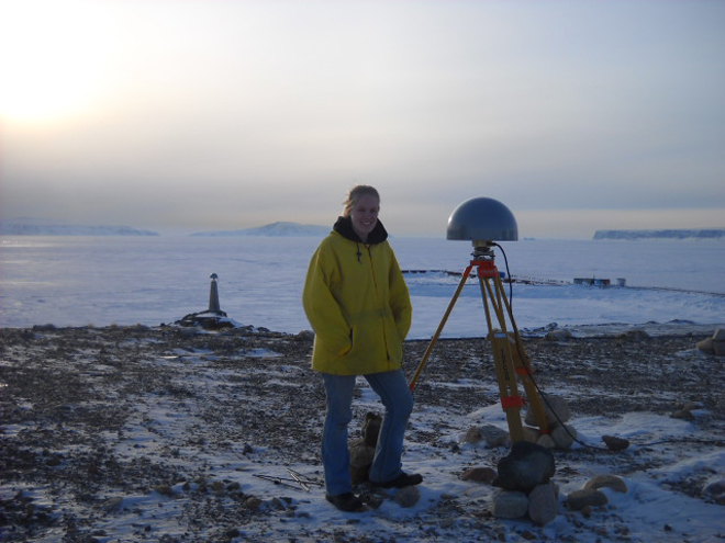
Markus: There are some measurements from drillings or from icebreakers, but those are snapshots in time and very sparse. The area you cover with a ship is excruciatingly small. So we do have some idea, but it’s not great. With the ICESat satellite and the Operation Ice Bridge airborne campaign, we have a chance to get ice thickness measurements over larger scales than we have been able to get before.
We have more instruments on the plane than we have on the satellite. So while aircraft don’t provide nearly the coverage of satellites, you do get additional information — such as thickness — that should be really useful.
What sea ice information will we get from the aircraft campaigns?
Markus: We have a laser altimeter, Bill Krabill’s instrument, that’s similar to ICESat and is the primary instrument of the mission. The laser bounces off the surface, whether it’s snow or ice, and provides a measure of surface elevation. But we also have radars on this plane, developed by the University of Kansas, which penetrate the snow. If you look at the difference between the laser and radar results, ideally you get the snow depth.
Accurate snow depth is important for estimating sea ice thickness, which is done with a conceptually simple calculation: if you know how much ice is above the water, then you can estimate how much is below the water. The problem occurs when you have snow on top, which submerges the ice to some extent.
Snow depth is a bigger issue for Antarctica because we have overall thinner ice and more snow than we have in the Arctic. It can vary quite significantly — anywhere from zero to a few meters — and it can be so heavy that the ice itself is submerged below sea level and you get flooding on the interface.
ICESat does not have radar, so in this regard we are getting a value-added product in Ice Bridge. In an ideal world, people would put a radar altimeter together with a laser altimeter — something you can do on a plane, but not as easily on a satellite.
So there’s a need to continue flying airplanes?
Markus: Yes. Some people are saying “Wow, we can do everything with airplanes,” which is wrong because the Antarctic is huge. It looks great on paper because all the flight lines that we draw on maps are pretty thick. But if you drive with your car across the United States and measure something, does this represent the entire United States? If you drive too far south, you miss the Rockies, and if you drive too far north, you miss the desert Southwest, so you get a completely wrong picture of the United States.
We can, however, look at critical areas in the sea ice, as well as over the ice sheets and see how they are changing in the time between ICESat and ICESat-II, so that we are not completely blind.
Why is it important to have that continuous coverage in Antarctica?
Markus: We want to establish a consistent long-term record so that we have continuous coverage. A gap in data leaves you with just a snapshot in time and poses a problem. For example, if you measured Washington, D.C.’s temperature in December 1990 at 70 F and then again on that date 10 years later at 30 F, you might assume a dramatic cooling trend. We want to avoid a similar misinterpretation of changes in Antarctica. We now have five years of data from ICESat, but we have just started to understand the processes.
Have you been to Antarctica?
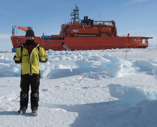
Markus: Yes, several times for field work. On an icebreaker mostly.
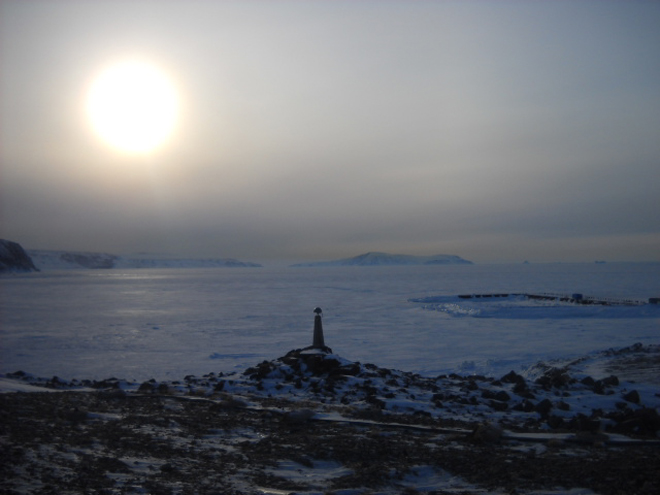
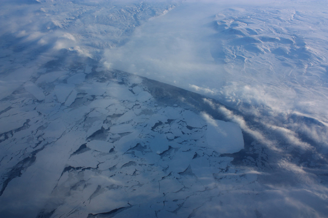
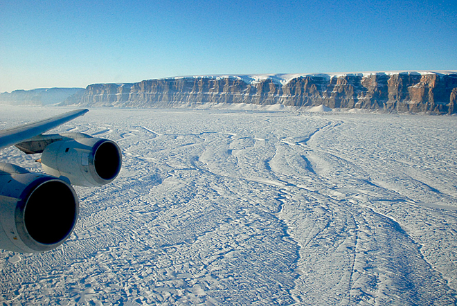
The irony is that from a plane, as well as from on the ice, it looks and feels like really solid ground. It looks perfectly still. You’re in an ice desert. On previous field expeditions that were on the ice, we would take out drills and hammers and more sophisticated instruments and do our work; it looks pretty much like a construction site. The captain would tell us afterward that we drifted 10 miles while we were working. It’s just incredible if you think about it: standing on ice we would measure its thickness with all these drills and know we were on 15-20 centimeters of ice, and that underneath is 4,000 meters of water. You’re floating out there, it’s a terribly cool thing.
What about from the sky?
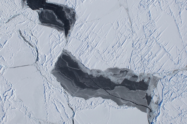
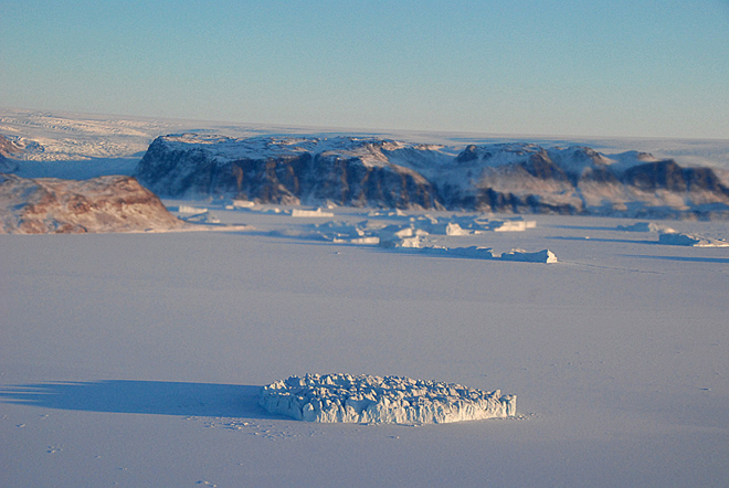
Markus: Ice Bridge flights won’t land in Antarctica, but even from a plane, sea ice looks static. An animation compiled from satellite images of Antarctic sea ice shows you how dynamic the sea ice is — how it looks like a living thing. In Greenland, I showed a similar movie of Arctic sea ice to the pilots while we were flying and they were amazed when they saw what’s really happening. Only since satellites did people get a better understanding how dynamic the sea ice is.
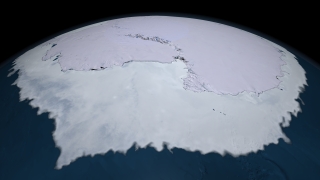
Sea ice surrounding the Antarctic landmass is dynamic, shifting in location, extent and thickness. This animation shows the sea ice motion around Antarctica from June 4 through Nov. 18, 2005. Credit: NASA/Goddard Space Flight Center Scientific Visualization Studio

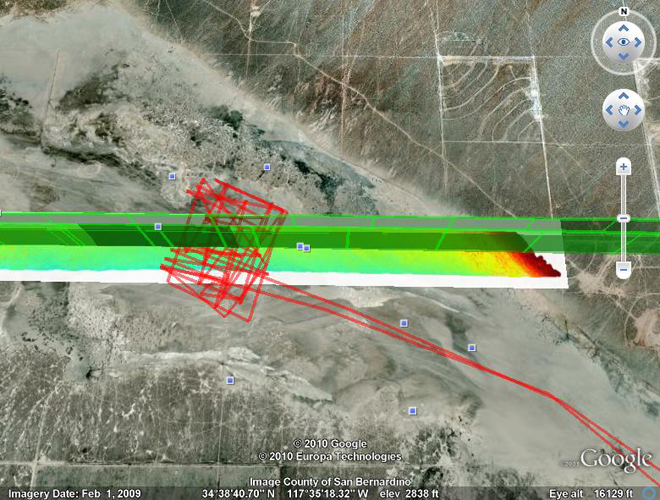


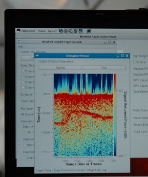 The display offers a cactus-like spectrum of color, with spikes protruding from separate layers of color. The uninitiated eye can clearly see a “surface” in the image. That would be the top of the ice layer, Allen explains. The more trained eye knows that where the yellow, aqua and blue colors intermingle is where the real action lies. More sophisticated methods will be needed to coax meaning from the raw data.
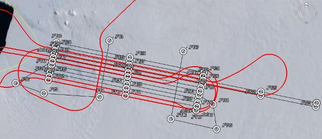
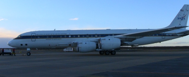
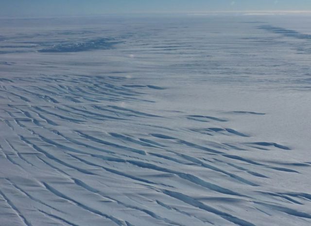
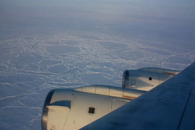
 On Sunday, Oct. 18, researchers and crew flew on the DC-8 aircraft’s second Antarctic flight of the Operation Ice Bridge Campaign. The mission was dedicated to reflying areas of Thwaites Glacier previously mapped by the ICESat satellite to see how the glacier has changed.
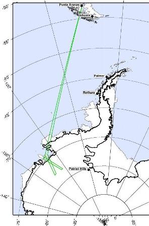
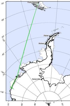 PUNTA ARENAS, CHILE – The first flight of Operation Ice Bridge was made from the southern tip of South America on Friday, Oct. 16. The primary target was the Getz Ice Shelf along Antarctica’s Amundsen Coast. The DC-8 flew two parallel tracks along the coast, one just offshore over the floating ice shelf, and one just inland. By measuring on either side of the “grounding line” between the floating ice and the ice on land, scientists can determine the rate at which this near-shore part of the ice shelf is melting.