From: Seelye Martin, University of Washington

The Weddell Sea mission is a pair of lines repeated from last year that extend across the sea ice from the tip of the Antarctic Peninsula to south of Cape Norvegia, and back again (see above). The flight path crosses the tip of the Peninsula, then proceeds on a long straight line to the eastern Weddell Coast, transits down the coast about 200 nautical miles, then transits back, where the sea ice coverage is at 1,500 feet. The primary instruments will be the ATM to measure sea ice freeboard and the snow depth radar for snow depth on the sea ice.
The past five days have been very difficult, in that the weather has been poor, with low clouds or storms over all of our sites. This was stressful for all of us, in that on the previous evening, we would choose a potential target, then get up at 5:00 am local, transit to the airport at 6:30, get to the airport at 7, stare at maps and imagery until 7:30, then consult with the weather office until 8 am. At this point, we would discover the weather was so marginal that we were forced to cancel. But today our forecasts showed a high pressure system over the Weddell Sea, the Chileans said go, so we flew the mission. This is the first in a series of 14 flight plans.
In this mission, our first problem involves the production of accurate weather forecasts. To produce these, we use the following sources: First, the Antarctic Mesoscale Prediction System, which at 00 and 12 UTC, produces a five day forecast at 3-hour increments. This forecast in particular shows the location and height of the cloud layers. Second, the satellite imagery acquired by the NASA Rapidfire system, pressure field forecasts from the European Center for Medium Range Weather Forecasting (ECMWF) and the expertise of Chilean Airport Meteorologists. So what’s the weather like down here? Imagine a circular icecap centered at the South Pole. Under these conditions, there would be a high pressure system over the ice cap, and a series of lows moving around the cap. Now add the Antarctic Peninsula to the icecap, a 4,000-meter-high barrier extending 700 nautical miles toward South America. The lows still rotate around the continent, but now the peninsula causes the lows to stall in the Bellingshausen Sea. This creates the bad weather for the critical region around Pine Island Bay. For the Weddell, this is the first open day since we arrived, and we hope that the mission is free of low clouds.
 A second problem involves the avoidance of bird and seal colonies. Low overflights stress the birds and seals; so we need to stay 4,000 feet away from the colonies in the vertical, or 1 nautical mile in the horizontal. We are making every effort to avoid the colonies, many of which are concentrated along our path in the northern peninsula.
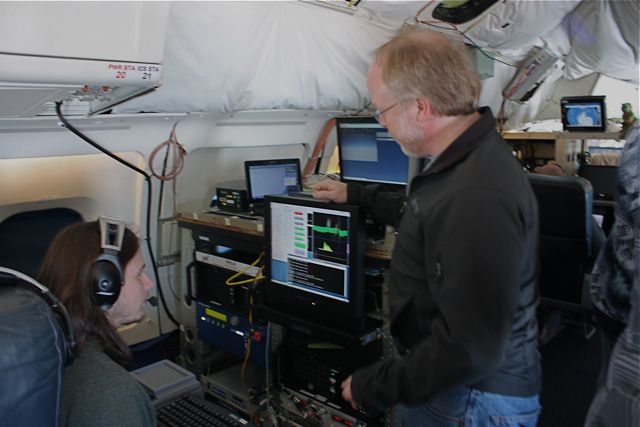
A third problem involves the snow depth radar. This is an innovative radar from the University of Kansas, that measures snow depth on sea ice. Last year, the transmit and receive antennas were located adjacent to one another in a fairing attached to the belly of the plane. This year, to improve performance, the receiving antennas were relocated to compartments in the wing roots, one each on each side. The relocation of these antennas involved having a contractor replace the aircraft aluminum panels with a radar transparent material, which is used instead of the aluminum panels, with the antennas mounted behind. The radar is now more sensitive, but it has yet to be tested over sea ice, something we had hoped to do on an earlier flight, so we need to allow for roughly half an hour to take data at low elevations, then analyze it, to make sure that the instrument is working properly before taking data along the line. Having this instrument work will improve the accuracy of the snow depth retrieval. So, weather, penguins, snow radar, all must all be considered for a successful flight.
Here is the timeline of the mission:
0905: Take-off to 33,000 ft, airspeed 450 kts.
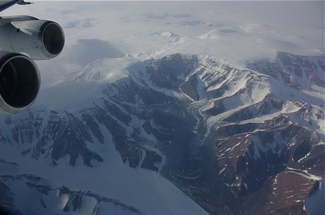
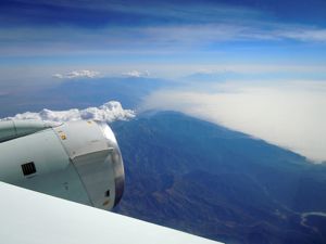
1030: We are approaching the peninsula, still at high altitude. Islands are just coming into view, poking up above the clouds, this would be Greenwich Island, straight ahead. Cloud deck is below us, clouds should clear as we cross the peninsula.
1026: Approaching peninsula, high clouds
1051: Passing over the peninsula at 34,000 ft, turbulence shakes plane.
1110: Cleared peninsula, avoided penguin colonies, sea ice is visible straight ahead, dropping our altitude to 1,500 ft. Someone just handed me a paper towel, they are concerned about possible precipitation inside the plane as we descend.
1112: Descending to 1500’ for snow radar calibration.
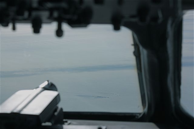
1113: At 1,500’, approaching sea ice under clouds, snow radar is running
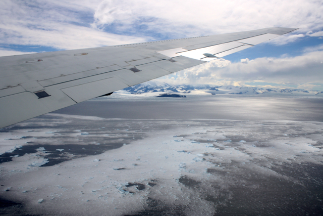
1115: Transiting sea ice edge. small broken floes, sunlight on ice. Surface temp from infrared radiometer is about -2 C. It is warm and sunny out here.
1146: Surface temp as low as -6C, we have good snow. Ice consists of large floes surrounded by open water, occasional nilas (thin ice). Small icebergs visible in distance. This is wonderful flying, horizon visible in all directions, blue sky above. Very different than last year. Gives some faith to the forecast.
1201: Suddenly flying above dense low clouds without breaks.
1208: Dropped to 1,000 ft, still in clouds, some turbulence. I sure hope we fly out of this.
1217: Intermittent cloudiness, now appears to be sharpening up. Pilots do not want to go below 1,000 ft. Now it is really clear again, a whole lot better.
1219: Looks really clear again, good horizon, occasional puffs of clouds, blue sky overhead.
1225: Winds up to 25 kts at right angles to the plane, Langmuir streaks in water. Winds should blow the clouds out of here. Ben reports that the snow radar is working.
1230: Return to 1,500 ft.
1311: Cross-track wind up to 31 kts.
1318: Clouds at horizon, 2 hours to the coast. Ice and blue sky still present.
1350: We are about an hour out from the eastern Weddell coast.
1400: Back into low clouds, some chop, wispy ground fog is back, surface still visible at times, still at 1,500 ft.
1413: Clear again at surface, but overcast overhead. 26 minutes to end of line. Losing the horizon. Turbulence, socked in again, no, I can still see the surface. These cloudy interludes are pretty intermittent. Can sort of see the horizon. Ben reports from early processing of snow radar, 75 cm of snow depth near the peninsula.
1435: Approaching the coast for our turn south. Then about 200 nm on the southern leg, then head back to the peninsula.
1440: Begin turn to the southwest. This is about as close as we will get to the eastern Weddell coast, the British station Halley Bay is off here somewhere, looks like we are on the new trajectory. We are in a heavy haze, but surface is still visible. Good surface visibility.
1530: Just finished traverse along the Brunt ice shelf, very beautiful as we came out from under a cloud deck.
1552: On return track to the tip of the peninsula, good surface visibility but hazy.
1700: Perfect weather on the return line, just heard from pilots that they can finish the line at 1,500 ft. Our low altitude airspeed is 250 knots.
1820: Approaching the peninsula at low altitude, weather remains excellent, beautiful sunset across the Peninsula.
1840: 15 minutes out from waypoint marking the end of the line. We can just about make out the Antarctic Peninsula. Ice is thicker adjacent to the peninsula, this is where the second year ice occurs in the Weddell Sea. The tabular icebergs we are seeing out here probably calf off the Ronne/Filchner Ice Shelves.
1850: Reached waypoint, starting to climb for home, at a sufficient altitude to avoid the penguin colonies.
1900: Cleared the peninsula, at 34,000 ft, headed for home, but encountered 60 kt headwinds.
2120: Landed at Punta Arenas, flight duration was 12.4 hrs.
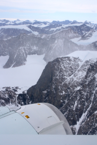 Stomachs also suffered from the dramatic changes in altitude necessary to collect data. The measurements require a relatively consistent altitude, which can be tricky when accessing a glacier behind a rock cliff. But the pilots deftly handled the 7,000-foot-roller coaster flight line to collect data over targets also surveyed during the 2009 campaign.


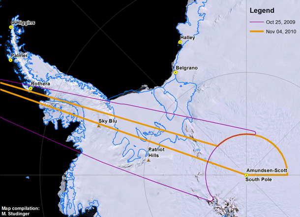
 3:50 PM – Now we’re heading on a straight line from the South Pole, following the exact track we did a few days ago, just before I arrived in Punta Arenas, in order to mimic the ATM swath and compare datasets.
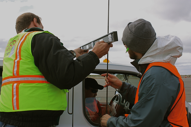


 Oct. 30, 2010


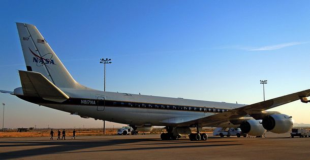
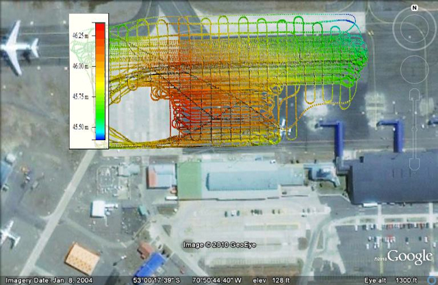
 But before we can go south we have to go through a series of test flights here in California to make sure that all the installed sensors work and to calibrate our science instruments. In order to do this we fly over target sites in the Mojave Desert that we have surveyed on the ground a few days before the test flights. The desert environment that we have selected for our test flights here is very different from the barren land of snow and ice that we will be flying over the next couple of weeks and we all enjoy the low altitude flights over the Mojave Desert, the San Gabriel Mountains and the San Andreas Fault. When the pilots ask you if it would be a problem if the belly of the aircraft is facing the sun you know that you are in the world of research flying. We did a couple of 90 roll maneuvers at high altitude over the Pacific Ocean to calibrate the antennas of the ice-penetrating radar systems that we will use to survey sea ice, glaciers, and ice sheets.
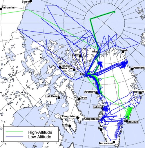
 IceBridge project scientist